
As mentioned before, geometric models in OpenSCAD are described by a textual description. At first glance, this description resembles a program written in a programming language such as Javascript or C. Especially if you have some programming experience, this apparent similarity can lead to some misunderstandings and misguided intuitions. Although the textual description reminds of classical program code, it is not a program. Rather, it is the specification of a geometric structure. In the course of the following sections, this difference will become more apparent. The focus of this chapter lies on conveying the essential concepts and functionality of OpenSCAD using select examples. An exhaustive description of all functions can be found at the end of the book as well as in the online documentation of OpenSCAD.
Let’s start by describing our first geometry in OpenSCAD. If you have not already done so, now would be a good time to start OpenSCAD with an empty or new file. The OpenSCAD program window should show the internal editor, the output window and the console view. You can hide the Customizer for now.
The basis of any geometry in OpenSCAD are so-called primitives. These are two or three dimensional basic shapes that we can use as building blocks for our model. Let’s create a simple sphere. To do this, enter the following into the editor:
sphere(10);If you now run a preview (F5), the output window should show a sphere with a radius of 10 millimeters.
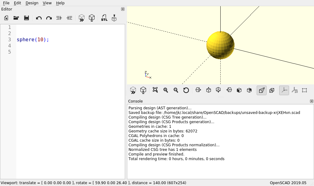
Also take a look at the console window. You should find a number of messages that were generated as part of the preview. The second to last line of this output should contain the message Compile and preview finished. (Figure 2.).
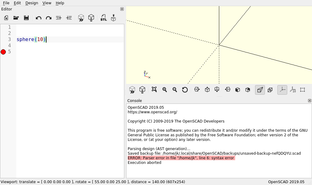
If instead there is a red marked ERROR in the console output, something went wrong (Figure 2.). Maybe you mistyped? Or maybe you forgot the semicolon at the end of the line? Did you perhaps write sphere with a capital S instead of a small one? Try to find the mistake and run the preview (F5) again.
Each basic shape in OpenSCAD has a unique name, which is always followed by a list of parameters in round brackets and a terminating semicolon. In the example above, the radius of the sphere is the first parameter. Each parameter also has a name and in general it is better to include this name. In the case of the sphere, the radius parameter has the name r and using this parameter name would look like this:
sphere(r = 10);Even if it requires a bit more typing effort, using the parameter name has two advantages. First, the geometry description becomes more readable. Second, you don’t have to remember the exact order of the parameters in case a basic shape has multiple ones. This is also the case with the sphere. Instead of the radius, you can also define a sphere by giving it a diameter:
sphere(d = 10);Try it out (F5). The sphere should now appear with only half of its previous size in the output window. What will happen if we specify both a radius and a diameter?
sphere(r = 10, d = 10);If you now run a preview (F5), then the sphere does not change and a warning highlighted in yellow is displayed in the console: Ignoring radius variable ‘r’ as diameter ’d' is defined too. So for the sphere, the diameter has priority over the radius if both are given. The order of the parameters does not matter here.
If you have some programming experience, the expression sphere(r=10); may remind you of a method call. Unfortunately, in the context of OpenSCAD this intuition is more hindering than useful. It is better to interpret the expression not as a method call, but rather as a statement about the existence of a concrete geometry. In this sense, the expression sphere(r=10); says something like: there exists a sphere with radius 10mm.
So far we have specified the radius of our sphere with a concrete value. If we are sure that we will never need or want to adjust this value again, this is perfectly fine. However, if we want to make the radius of the sphere configurable in our model, then we should give the radius its own name. We can do this by using a variable:
radius_with_a_name = 10;

sphere( r = radius_with_a_name );
In larger projects it is useful to collect all configuration variables at the beginning of the model file. This way, you have an overview of all possible settings. In addition, you should get into the habit of commenting the variables (and the geometry where it feels suitable) right away. Single-line comments can be introduced with //. In this case, everything up to the end of the line is considered a comment. If you need more space, you can start a comment block with /* and end it with */:
/*
    This is an OpenSCAD test project
    --------------------------------
*/

radius_with_a_name = 10;  // a very important radius

// the main sphere of our model
sphere( r = radius_with_a_name );
At this point programming experience can be a hindrance again. Our model looks even more like a typical sequential program now! But this is not the case. A variable in OpenSCAD represents not a memory location that could take on different values in the course of a program. Instead, it is again just an existence statement: there exists the value 10 called “radius_with_a_name”. What happens if we assign a value to a variable twice? Let’s try it out!
radius_with_a_name = 10;

sphere( r = radius_with_a_name );

radius_with_a_name = 20;
If we now run the preview (F5), we see that the sphere is rendered with a radius of 20. At the same time we see a warning in the console output: sphere radius was assigned on line 1 but was overwritten on line 5. As you can see, you can only give one value to a variable. OpenSCAD always uses the last value that was assigned (here 20). This also means that a variable does not have to be defined “before” it is used. The “before” is in quotes because there is no temporal “before” in this sense in an OpenSCAD geometry description.
When describing values by variables, one is not limited to using only single values. Let’s assume that the dimensions in our model still need a correction value. We could implement this like so:
adjustment = 0.7;

main_radius = 10 + adjustment;
margin      =  5 + adjustment;
depth       = 25 + adjustment;

// ... even more configuration variables with adjustment
So far so good. Let’s assume that we suddenly realize that we also need a correction factor! We could implement that as follows:
adjustment        = 0.7;
adjustment_factor = 1.05;

main_radius = (10 + adjustment) * adjustment_factor;
margin      = ( 5 + adjustment) * adjustment_factor;
depth       = (25 + adjustment) * adjustment_factor;
You can already see that it’s kind of cumbersome to have to update every configuration variable. A more elegant solution is to use a function for the adjustment:
adjustment        = 0.7;
adjustment_factor = 1.05;

function adjust(x) = (x + adjustment) * adjustment_factor;

main_radius = adjust(10);
margin      = adjust( 5);
depth       = adjust(25);
If we now need to change the adjustment in our example again, then we only need to update the function adjust(x). Function definitions are introduced with the keyword function, followed by a unique name for the function (here adjust) and a parameter list in round brackets (here (x)). The function itself is written after an equal sign and always ends with a semicolon. Apart from our own custom functions, OpenSCAD offers a whole set of predefined functions (e.g. sin(), cos(), round()), most of which we will get to know within the course of this book.
Before we move on to the next section, let’s briefly recap what we have learned:
In the previous section we used the basic shape sphere in our model description. Now, for a change, we will use a cube:
cube(size = 10, center = true);The parameter size sets the length of the cube’s edges. The parameter center defines where the cube has its origin (Figure 2.).
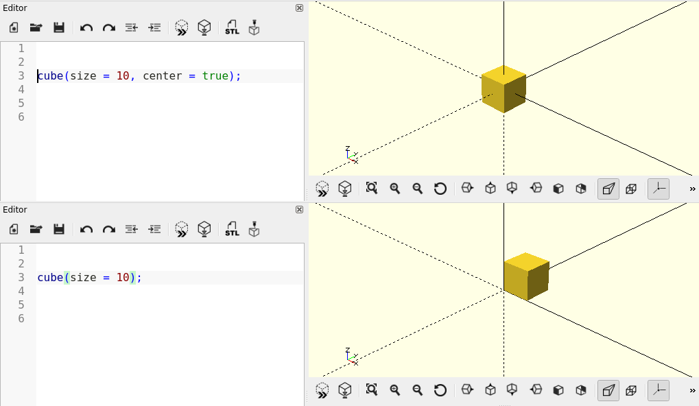
Like the sphere, the cube is displayed at the origin of the coordinate system. In the output window, the coordinate system is represented by three perpendicular lines, each representing the X-, Y- and Z-axes, respectively. The positive regions of each axis are represented by solid lines. The negative regions are represented by dashed lines. With the shortkey ‘CTRL + 2’ the coordinate axes can be shown or hidden. Also, pay attention to the small, labeled coordinate cross at the bottom left of the output window. It serves as an orientation aid.
If we now want to move our cube to another position, we have to use a so-called transformation. In this case a translation:
translate( [20,0,0] ) cube(10,true);A transformation (here translate( [20,0,0] )) always affects the following element. In this case our cube. The transformation translate gets a three-dimensional vector as parameter, which describes the desired displacement in X-, Y- and Z-direction. Vectors are written with square brackets in OpenSCAD and the numbers inside a vector are separated by commas.
It is important to emphasize a key concept of the OpenSCAD language here: The entire expression translate(...) cube(...); is an independent geometric object that can be used like any other basic shape (sphere, cube, etc.)! This means, in particular, that we can prepend further transformations to this new object, e.g. a rotation:
rotate( [0,0,45] ) translate( [20,0,0] ) cube(10,true);The transformation rotate rotates a geometric object around the origin. As parameter the transformation requires a three-dimensional vector. In this case the vector contains the desired rotation angles around the X, Y and Z axis. And again, the entire expression rotate(...) translate(...) cube(...); is a new, independent geometric object. Since the semicolon marks the end of that object, you can also write the transformations in the lines above the basic shape (here: cube) to avoid an overly long line length.
Figure 2. illustrates how our final result depends on the order of the transformations. Since the transformations in OpenSCAD always refer to the origin, it makes a big difference whether you move an object first and then rotate it, or vice versa.
Basic geometric shapes and transformations give us roughly the modeling capabilities that we had as children with our toy building blocks. In the next section, we will expand these capabilities significantly.
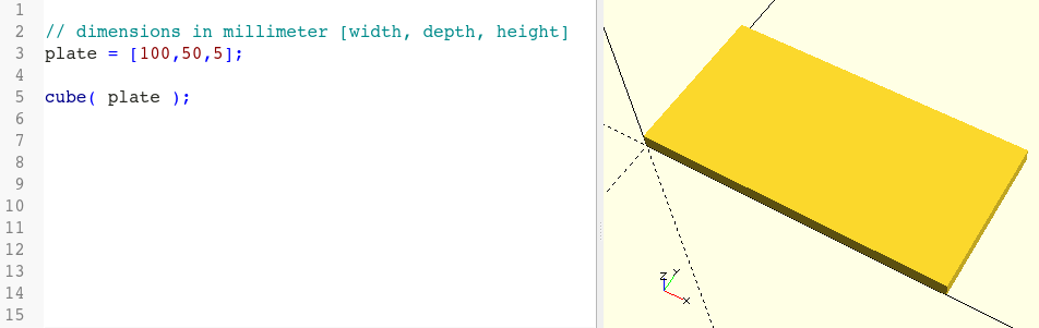
Let’s assume that we want to model a 5mm thick plate with a dimension of 10cm x 5cm. We could do this as follows:
// dimensions in millimeter [width, depth, height]
plate = [100,50,5];

cube( plate );
We define a three-dimensional vector plate containing the dimensions of our plate and pass this vector as a parameter to the basic shape cube (Figure 2.).
Suppose we now want to model four holes at the corners of the plate. Let’s start by defining two variables. One for the diameter of the holes and one for the distance of the holes from the edge of the plate:
// dimensions in millimeter [width, depth, height]
plate = [100,50,5];

hole_dm     = 6;
hole_margin = 4;

cube( plate );
Next, we need to describe what shape our holes should have. The basic shape cylinder is suitable for this:
// dimensions in mm [width, depth, height]
plate = [100,50,5];

hole_dm     = 6;
hole_margin = 4;

cube( plate );

cylinder( d = hole_dm, h = plate.z );
The parameter d of the basic shape cylinder sets the diameter, the parameter h sets the height. We pass our variable hole_dm as d and the Z-coordinate of the plate vector as h, as plate.z contains the thickness of our plate. Instead of plate.z we could have written plate[2] as well.
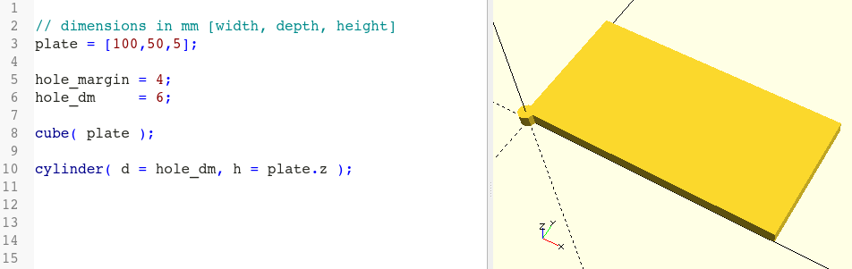
The cylinder has now the right dimensions but is still in the wrong place (Figure 2.). Moreover, it is hard to distinguish from the plate. Let’s move the cylinder and give it a different color:
// dimensions in mm [width, depth, height]
plate = [100,50,5];

hole_dm     = 6;
hole_margin = 4;

cube( plate );

translate
([
	hole_margin + hole_dm / 2,
	hole_margin + hole_dm / 2,
	0
])
color( "red" )
cylinder( d = hole_dm, h = plate.z );
First, we apply the transformation color and use it to color the cylinder red. We then move the red cylinder to the lower left corner of the plate using the transformation translate. To keep our model description a bit clearer, we have arranged the parameter of the translate transformation vertically.
Before we take care of the cylinders needed in the other three corners, we create our first hole in the plate. This is done with a so-called Boolean operation, which can combine two or more geometries. In OpenSCAD there are three types of Boolean operation available: difference, union, and intersection. For our hole we need the difference operation because we want to “subtract” the cylinder from the plate:
// dimensions in mm [width, depth, height]
plate = [100,50,5];

hole_margin = 4;
hole_dm     = 6;

difference() {

	cube( plate );

	translate
	([
		hole_margin + hole_dm / 2,
		hole_margin + hole_dm / 2,
		0
	])
	color( "red" )
	cylinder( d = hole_dm, h = plate.z );

}
Just like a transformation, a Boolean operation (here: difference()) affects the following element. Since Boolean operations combine multiple geometries, it would make little sense if the subsequent element consisted of only a single geometry - even though this would be valid in principle. To have more than one subsequent element a geometry set is used. It is defined by enclosing one or more geometric objects with a pair of curly braces { ... }. In case of the difference operation all geometries following the first geometry in the set are subtracted from that first geometry.
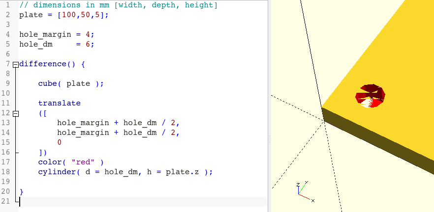
Figure 2. shows that our first hole is, unfortunately, not without errors. The surface at the location of the hole shows strange defects. Especially when you change the view in the output window with the mouse. These defects are caused by rounding errors during the difference calculation, as the top and bottom sides of our cylinder are flush with the top and bottom side of the plate. To fix the problem, we need to increase the height of the cylinder a tiny bit while at the same time move it down a bit so that the cylinder protrudes both top and bottom of the plate:
// dimensions in mm [width, depth, height]
plate = [100,50,5];

hole_dm     = 6;
hole_margin = 4;

difference() {

	cube( plate );

	translate
	([
		hole_margin + hole_dm / 2,
		hole_margin + hole_dm / 2,
		-1
	])
	color( "red" )
	cylinder( d = hole_dm, h = plate.z + 2);

}
Now the resulting hole looks clean (Figure 2.). To check the position of the cylinder you can temporarily prefix the cylinder object with a # in the model description and re-run the preview. This will display the cylinder with a semi-transparent red color.

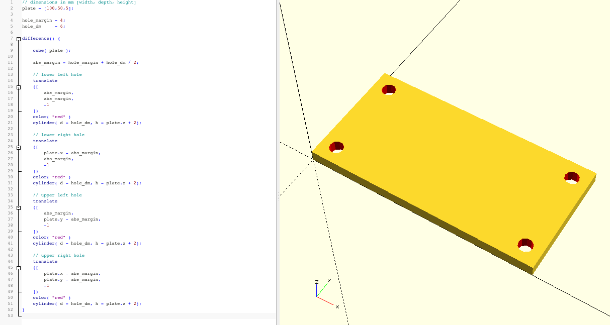
Now we can finally take care of the other three holes. To do this, we simply copy our existing cylinder three times and adjust the position in each case:
// dimensions in mm [width, depth, height]
plate = [100,50,5];

hole_dm     = 6;
hole_margin = 4;

difference() {

	cube( plate );

	abs_margin = hole_margin + hole_dm / 2;

	// lower left hole
	translate
	([
		abs_margin,
		abs_margin,
		-1
	])
	color( "red" )
	cylinder( d = hole_dm, h = plate.z + 2);

	// lower right hole
	translate
	([
		plate.x - abs_margin,
		abs_margin,
		-1
	])
	color( "red" )
	cylinder( d = hole_dm, h = plate.z + 2);

	// upper left hole
	translate
	([
		abs_margin,
		plate.y - abs_margin,
		-1
	])
	color( "red" )
	cylinder( d = hole_dm, h = plate.z + 2);

	// upper right hole
	translate
	([
		plate.x - abs_margin,
		plate.y - abs_margin,
		-1
	])
	color( "red" )
	cylinder( d = hole_dm, h = plate.z + 2);
}
The geometry set of the difference operation now contains five objects. Our plate followed by four cylinders. This leads to the desired result (Figure 2.). However, our geometry description is now very extensive and somewhat convoluted.
Whenever you find yourself copying a definition block multiple times, only to change it minimally each time, you have a strong indication that there is probably a better way to describe the current geometry. This is also true here. Instead of copying the cylinders four times, we can describe the four instances using a loop:
// dimensions in mm [width, depth, height]
plate = [100,50,5];

hole_dm     = 6;
hole_margin = 4;

difference() {

	cube( plate );

	abs_margin = hole_margin + hole_dm / 2;
	x_values   = [abs_margin, plate.x - abs_margin];
	y_values   = [abs_margin, plate.y - abs_margin];

	// holes
	for (x = x_values, y = y_values)
    translate( [x, y, -1] )
    color( "red" )
    cylinder( d = hole_dm, h = plate.z + 2);

}
Loops in OpenSCAD begin with the keyword for followed by the definition of one or more loop variables in round brackets. The loop variables can be assigned either an array or a range. We have already learned about arrays in the form of vectors. They do not differ in their definition. A range looks very similar to an array: [start_value : end_value] or [start_value : increment : end_value]. You can think of a range as an implicit array where you only specify start and end values while the values in between are calculated automatically. If no increment is specified, an increment of 1 is assumed.
Just like transformations and Boolean operations, for-loops operate on the subsequent element, which is used as a template to create a new geometric object for each possible combination of the loop variables. At those places where the loop variables are used in the template, the corresponding values from the associated array or range are substituted. The “result” of a for-loop is not a geometry set, but a single, unified geometry.
Our example uses the x_values and y_values arrays, which are assigned to the loop variables x and y. Here is a version that uses two ranges:
// dimensions in mm [width, depth, height]
plate = [100,50,5];

hole_dm     = 6;
hole_margin = 4;

difference() {

	cube( plate );

	abs_margin  = hole_margin + hole_dm / 2;
	x_hole_dist = plate.x - 2 * abs_margin;
	y_hole_dist = plate.y - 2 * abs_margin;
	x_values    = [abs_margin : x_hole_dist : plate.x - abs_margin];
	y_values    = [abs_margin : y_hole_dist : plate.y - abs_margin];

	// holes
	for (x = x_values, y = y_values)
    translate( [x, y, -1] )
    color( "red" )
    cylinder( d = hole_dm, h = plate.z + 2);

}
Using two ranges is a bit more involved than using two arrays as we have to calculate the appropriate increments x_hole_dist and y_hole_dist first. In the next section we will benefit from this extra effort. Before we continue it is worth having a look at the Customizer (Figure 2.).
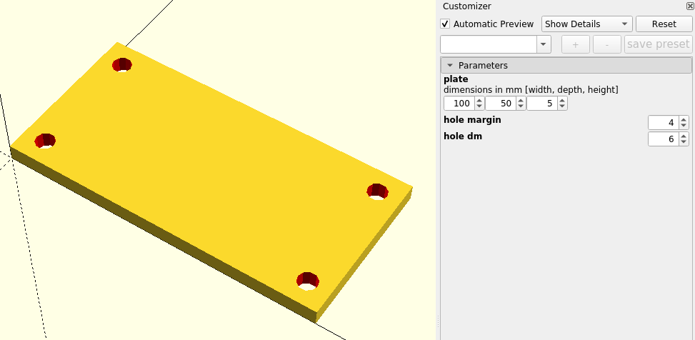
Our variables plate, hole_dm and hole_margin were automatically recognized and inserted as controls in the Customizer. If the Customizer does not show anything, it helps to let the preview run again. Click on the small triangle in front of Parameters if necessary. You can now save and load different configurations as Presets. However, this functionality only works if you have already saved the geometry description as a .scad file. The presets themselves are saved in a second file, which has the same name as the .scad file, but ends in .json.
The geometry description of our plate is now pretty much finished. What we are still missing is the ability to use our plate multiple times without having to copy our geometry description. For this purpose we can package a geometry description inside a module:
module hole_plate( size, hole_dm, hole_margin) {

	difference() {

		cube( size );

		abs_margin  = hole_margin + hole_dm / 2;
		x_hole_dist = size.x - 2*abs_margin;
		y_hole_dist = size.y - 2*abs_margin;
		x_values    = [abs_margin : x_hole_dist : size.x - abs_margin];
		y_values    = [abs_margin : y_hole_dist : size.y - abs_margin];

		// holes
		for (x = x_values, y = y_values)
	    translate( [x, y, -1] )
	    color( "red" )
	    cylinder( d = hole_dm, h = size.z + 2);

	}

}

hole_plate( [100,50,5], 6, 4 );

translate( [0,60,0] )
hole_plate( size = [50,50,5], hole_dm = 3, hole_margin = 2 );

translate( [60,60,0] )
hole_plate( [50,50,5], hole_dm = 5, hole_margin = 5 );
In OpenSCAD a module definition starts with the keyword module. It is followed by the name of the module (here: hole_plate) and its parameter list in round brackets. We do not have to specify what type the parameters have. The type of the parameters is automatically determined by OpenSCAD based on their usage. Thus, in our example, the parameter size is a three-dimensional vector, while hole_dm and hole_margin are simple numbers. The content of a module is a geometry set enclosed by curly brackets - just as we have already seen with Boolean operators.
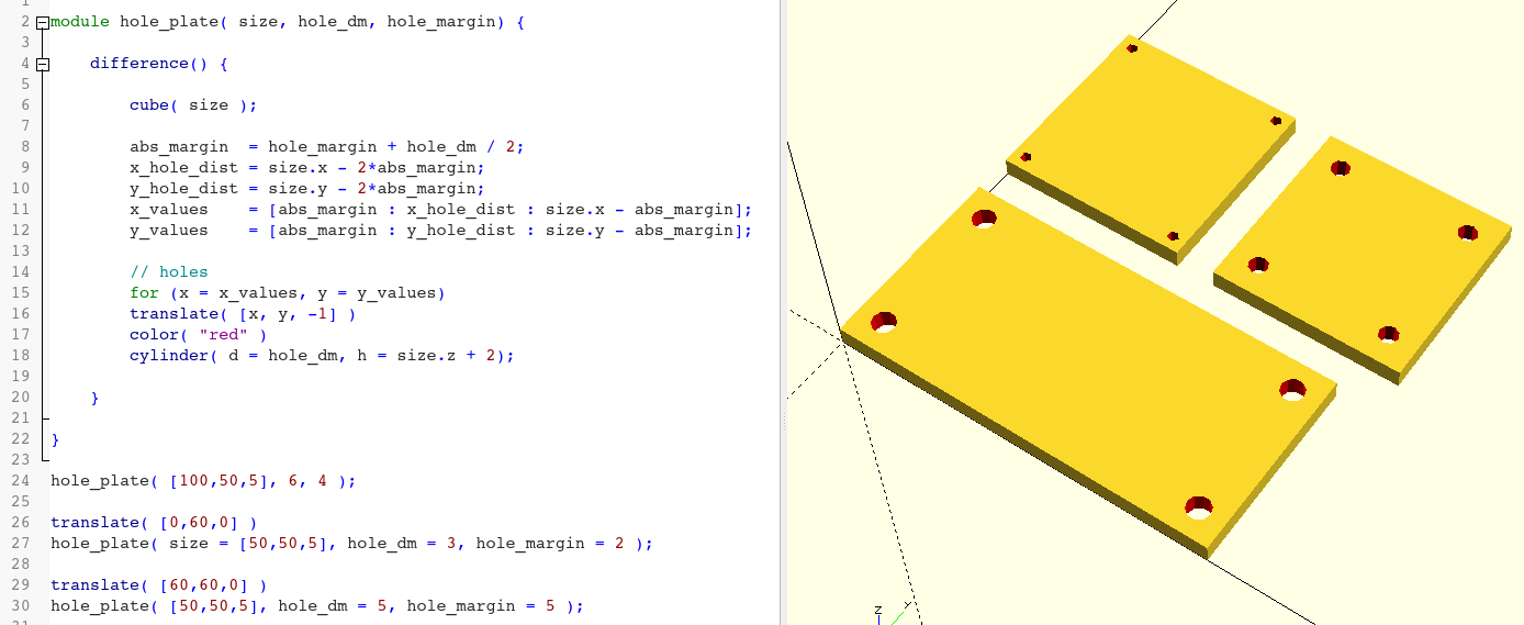
Once you have defined the module, you can use it like one of the basic shapes (sphere, cube, etc.). In our example, we have created three plates, two of which we have arranged using translate transformations (Figure 2.).
Within the module, we have taken our original geometry description and merely made the formerly global variables the module’s parameters. We used the last version of our description from the previous section. It allows us to easily extend the functionality of our module such that we can parameterize the number of holes:
module hole_plate( size, hole_dm, hole_margin, hole_count = [2,2] ) {

	difference() {

		cube( size );

		abs_margin  = hole_margin + hole_dm/2;
		x_hole_dist = (size.x - 2*abs_margin) / (hole_count.x - 1);
		y_hole_dist = (size.y - 2*abs_margin) / (hole_count.y - 1);
		x_values    = [abs_margin : x_hole_dist : size.x - abs_margin + 0.1];
		y_values    = [abs_margin : y_hole_dist : size.y - abs_margin + 0.1];

		// holes
		for (x = x_values, y = y_values)
	    translate( [x, y, -1] )
	    color( "red" )
	    cylinder( d = hole_dm, h = size.z + 2);

	}

}

hole_plate( [100,50,5], 6, 4 );

translate( [0,60,0] )
hole_plate(
	size        = [50,50,5],
	hole_dm     = 3,
	hole_margin = 2,
	hole_count  = [4,6]
);

translate( [60,60,0] )
hole_plate( [50,50,5], hole_dm = 5, hole_margin = 5, hole_count = [4,3] );
We have added a parameter hole_count to our module and given it a default value (here: [2,2], a two-dimensional vector). Since we used two ranges (x_values and y_values) for the loop variables, we only need to adjust the increments x_hole_dist and y_hole_dist to create the desired number of holes in X- and Y-direction. Again, rounding errors can get in our way. Therefore we also have to adjust the end value of the ranges slightly (+ 0.1). As the actual values used in the for-loop are determined solely on the basis of the increments, we do not cause any inaccuracy in our design with this adjustment.
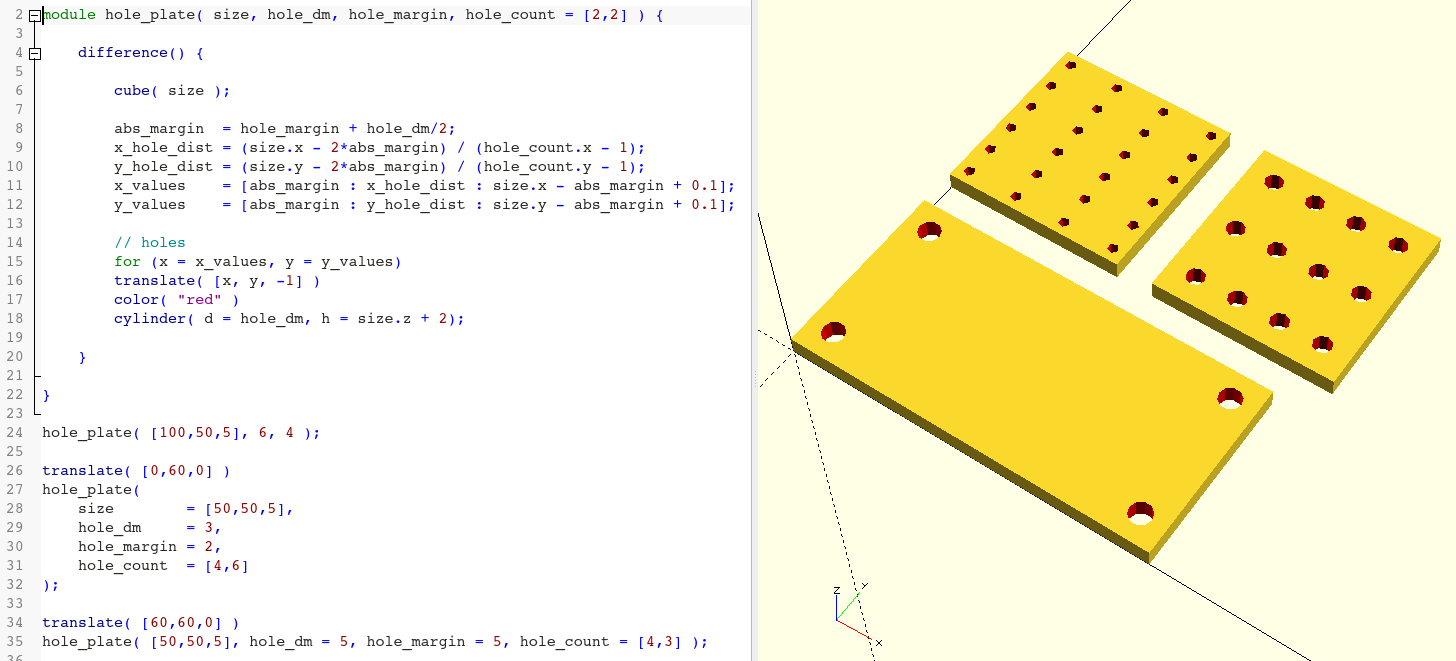
Since we have defined the new hole_count parameter of our module with a default value, the module is “backwards compatible”. Thus, the first use of our module, in which we do not specifiy a value for hole_count, has not changed (Figure 2.).
Our module still has a few blemishes. If the parameter hole_count contains the value 1, then the calculation of the corresponding hole distance contains a division by 0. This is not good and we should definitely take care of it. Maybe we should just make a single, centered hole if count is 1? To achieve this, we need to make both the calculation of the hole distances (x_hole_dist and y_hole_dist) and the definition of the value ranges (x_values and y_values) conditional on the hole_count parameter:
module hole_plate( size, hole_dm, hole_margin, hole_count = [2,2] ) {

	difference() {

		cube( size );

		abs_margin  = hole_margin + hole_dm / 2;

		x_hole_dist = hole_count.x > 1 ?
		              (size.x - 2 * abs_margin) / (hole_count.x - 1) : 0;

		y_hole_dist = hole_count.y > 1 ?
		              (size.y - 2 * abs_margin) / (hole_count.y - 1) : 0;

		x_values    = hole_count.x > 1 ?
					  [abs_margin : x_hole_dist : size.x - abs_margin + 0.1] :
				  	  [size.x / 2];

		y_values    = hole_count.y > 1 ?
		              [abs_margin : y_hole_dist : size.y - abs_margin + 0.1] :
		              [size.y / 2];

		// holes
		for (x = x_values, y = y_values)
	    translate( [x, y, -1] )
	    color( "red" )
	    cylinder( d = hole_dm, h = size.z + 2);

	}

}

hole_plate( [100,50,5], 6, 4 );

translate( [0,60,0] )
hole_plate(
	size        = [50,50,5],
	hole_dm     = 3,
	hole_margin = 2,
	hole_count  = [1,1]
);

translate( [60,60,0] )
hole_plate( [50,50,5], hole_dm = 5, hole_margin = 5, hole_count = [2,1] );
The conditional parts of the geometry description use the question mark operator. In general, this operator has the structure a ? b : c. The part a is always a yes or no question (here: “is hole_count.x greater than 1”). If the answer is yes, part b is taken as value, if the answer is no, part c is taken instead.
If you have some programming experience, you may have first thought about using an if statement to make the above case distinction. Again, “normal” programming intuition is a hindrance here. After all, we can only assign a value once to a variable in OpenSCAD! The following expression would therefore not work as expected in OpenSCAD:
x_hole_dist = 0;
if (hole_count.x > 1) {
	x_hole_dist = (size.x - 2 * abs_margin) / (hole_count.x - 1);
}
Nevertheless, there are also if-statements in OpenSCAD. You can use it to include or exclude whole parts of the geometry description. We can use it in our example to remove yet another flaw in our module. At the moment, a number of 0 or any negative value would also result in a single hole. This doesn’t seem to make sense. If we specify a 0 for the number of holes, then we obviously don’t want a hole at all:
module hole_plate( size, hole_dm, hole_margin, hole_count = [2,2] ) {

	if (hole_count.x == 0 || hole_count.y == 0) {

		cube( size );

	} else {

		difference() {

			cube( size );

			abs_margin  = hole_margin + hole_dm / 2;

			x_hole_dist = hole_count.x > 1 ?
			              (size.x - 2 * abs_margin) / (hole_count.x - 1) : 0;

			y_hole_dist = hole_count.y > 1 ?
			              (size.y - 2 * abs_margin) / (hole_count.y - 1) : 0;

			x_values = hole_count.x > 1 ?
					   [abs_margin : x_hole_dist : size.x - abs_margin + 0.1] :
					   [size.x / 2];

			y_values = hole_count.y > 1 ?
			           [abs_margin : y_hole_dist : size.y - abs_margin + 0.1] :
			           [size.y / 2];

			// holes
			for (x = x_values, y = y_values)
		    translate( [x, y, -1] )
		    color( "red" )
		    cylinder( d = hole_dm, h = size.z + 2);

		}

	}
}

hole_plate( [100,50,5], 6, 4 );

translate( [0,60,0] )
hole_plate(
	size   = [50,50,5],
	hole_dm   = 3,
	hole_margin = 2,
	hole_count    = [0,1]
);

translate( [60,60,0] )
hole_plate( [50,50,5], hole_dm = 5, hole_margin = 5, hole_count = [2,1] );
So here we distinguish right at the beginning whether we want to model a plate with or without holes and branch our geometry description accordingly. Equality is expressed with the double equal sign (==). The two vertical lines (||) have the meaning of a logical “or” in the sense of “only one of the two questions must be answered with yes”.
Let’s say we want to reuse our plate in another project. It would be a bad idea to simply copy the geometry description into the new project file. Instead, OpenSCAD offers two commands to include other .scad files into a project:
include <hole_plate.scad>;The include command imports another .scad file (here: hole_plate.scad) completely into the current geometry description. This means that also the three test plates we defined below our module would appear in the new geometry description. To avoid this, OpenSCAD also has the use command as an alternative:
use <hole_plate.scad>;If you import geometry with use instead of include, only the modules and functions from the other .scad file are imported, but no global variables or instantiations of geometries. The file specified within the angle brackets must either be located in the same directory as the file of the current geometry description, or in the Library Folder of OpenSCAD. You can use the menu entry File -> Show Library Folder to display the library folder and store your geometry libraries there. On the Internet you can find a number of very excellent geometry libraries for OpenSCAD. The library directory is the place where you have to copy them in order to use them.
If you want to use an external geometry in OpenSCAD that has a different format than .scad, you can use the import keyword.
import("logo.svg");The imported geometry can then be used like a basic shape (sphere, cube, etc.) or a module (e.g. translate(...) import("logo.svg");). OpenSCAD supports DXF and SVG as two-dimensional formats and STL, OFF, AMF and 3MF as three-dimensional formats.
Congratulations! You now know all essential concepts and functionalities of OpenSCAD. Everything else is really “just” details. In the following projects, we will practice and deepen our understanding of these concepts and gradually work our way through the remaining functionality. You will see that your understanding of the material will gradually improve with each project, so that you will soon have a clear understanding of how to get from an idea to a finished geometry description.