
Parabolic reflectors are fascinating. They concentrate incident parallel light or electromagnetic radiation in a focal point. Satellite antennas or solar stoves make use of this property. In the other direction, when a light source sits in the focal point, a parabolic mirror can be used to create a parallel cone of light.
In this project we will create the geometry description for a parabolic reflector.
We will get to know the 3D basic shape polyhedron. It is basically the three-dimensional counterpart of the 2D basic shape polygon. Creating a polyhedron is easy in theory, but quite challenging in practice. Therefore, we will proceed step by step and focus solely on this one novelty in this project.
A parabola is characterized by the fact that all points on the parabolic surface have the same distance to a reference or base surface and a focal point. Figure 11. shows this relation for a single point p of the parabolic surface and the corresponding points b on the base surface and f, the focus point. It can be seen that the points p, b and f form an isosceles triangle and therefore the distance between p and f and the distance between p and b are equal.
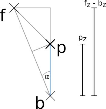
If we want to describe the geometry of a parabola, we need to determine the points p of the parabolic surface for a given focal point and a given base plane. If we look again at Figure 11., we see that point p lies vertically above point b. If we think of point b as part of a base surface in the X-Y plane, then we can simply take the X- and Y-coordinates of point p directly from point b. So only the Z-coordinate of p remains to be determined. Here two triangles can help us that are hidden in figure 11.. Both triangles share the angle α. The larger of the two has its hypotenuse from f to b and the adjacent f.z - b.z. The smaller triangle has as its hypotenuse the length p.z and as its adjacent exactly half the distance from f to b (because it is part of the isosceles triangle).
If we remember that cos(α) = adjacent / hypotenuse, it follows for the large triangle:
// distance between f and b
dist_fb = norm(f - b)

cos(α) = (f.z - b.z) / dist_fb
For the small triangle:
cos(α) = (dist_fb / 2) / p.zSince it is the same α in both cases, we can set the two ratios as equal and rearrange them to find the p.z we are looking for:
(f.z - b.z) / dist_fb = (dist_fb / 2) / p.z


// both sides times p.z

p.z * (f.z - b.z) / dist_fb = dist_fb / 2


// both sides divided by ((f.z - b.z) / dist_fb)

p.z = (dist_fb / 2) / ((f.z - b.z) / dist_fb)


// replace outer division by multiplikation with the inverse

p.z = (dist_fb / 2) * (dist_fb / (f.z - b.z))


// multiply out: numerator times numerator, denominator times denominator

p.z = (dist_fb * dist_fb) / (2 * (f.z - b.z))
With that, we are done! We now have a compact formula to calculate a point p on the parabolic surface with respect to a focus point and a base point. Let’s capture this result in an OpenSCAD function parabola_point:
function parabola_point( focus_point, base_point ) =
    let ( dist_fb = norm(focus_point - base_point) )
    [
        base_point.x,
        base_point.y,
        ( dist_fb * dist_fb ) / ( 2 * (focus_point.z - base_point.z) )
    ];
After these preparations we can start with the definition of a module parabola and calculate the points on the surface of the parabola with the help of our function parabola_point:
/*
    parabola module

    - focus_point,    focus point as 3D-vector
    - base_area,      dimension of the base are as 2D-vector
    - resolution,     number of grid points as 2D-vector
*/
module parabola( focus_point, base_area, resolution = [10, 10] ){

    function parabola_point( focus_point, base_point ) =
        let ( dist_fb = norm(focus_point - base_point) )
        [
            base_point.x,
            base_point.y,
            ( dist_fb * dist_fb ) / ( 2 * (focus_point.z - base_point.z) )
        ];

    parabola_points = [
        for (
            y = [0 : base_area.y / resolution.y : base_area.y + 0.1],
            x = [0 : base_area.x / resolution.x : base_area.x + 0.1]
        )
        parabola_point( focus_point, [x,y,0] )
    ];

}

parabola(
    focus_point = [75,75,100],
    base_area   = [150,150]
);
Our module parabola has three parameters. The parameter focus_point sets the position of the focus point of the parabola as a three-dimensional vector. The parameter base_area sets the dimension of the base surface in the form of a two-dimensional vector. Thus, we assume that our base surface is located with one corner at the origin and lies on the X-Y plane (Z = 0). The third parameter resolution sets the number of individual surfaces in the X- and Y-directions that the parabolic surface should consist of.
Inside the module we calculate the parabola_points as an array of vectors via a generative, two-dimensional for-loop. The step size of the loop variables results from the respective number of partial surfaces (resolution) and the dimension of the base surface (base_area). The addition of a tenth of a millimeter at the respective upper limits of the ranges serves to compensate for rounding errors. It does not mean that the parabola would become one tenth larger. Finally, inside the generative for loop, we use our function parabola_point to calculate each point of the parabola surface.
Since we want to create a three-dimensional body, we still need the points of the base surface itself. We can also create these with a generative for-loop. Instead of using a function like parabola_point, we can specify the three-dimensional vector of the points directly. It consists only of the X- and Y-coordinates and a constant Z-coordinate, which we set to 0:
module parabola( focus_point, base_area, resolution = [10, 10] ){

    /* ... */

    parabola_points = [
        for (
            y = [0 : base_area.y / resolution.y : base_area.y + 0.1],
            x = [0 : base_area.x / resolution.x : base_area.x + 0.1]
        )
        parabola_point( focus_point, [x,y,0] )
    ];

    base_points = [
        for (
            y = [0 : base_area.y / resolution.y : base_area.y + 0.1],
            x = [0 : base_area.x / resolution.x : base_area.x + 0.1]
        )
        [x, y, 0]
    ];

}
/* ... */
Now we come to a somewhat tricky part. We have to explicitly specify the individual surfaces of our geometry. Each individual surface needs four points, which have to be specified in order. This is basically like trying to trace the outer edge of the surface with a pencil all the way through without starting over. You may remember these puzzle pictures in your childhood. You were given a sheet of paper with numbered dots and then you had to connect the dots one by one to reveal the picture. We’re doing something similar now.
The points in our arrays parabola_points and base_points lie one after another as a long list. Each of these lists contains (resolution.x + 1) * (resolution.y + 1) points. Thus, you can identify each point with a number. Just like the house numbers along a street. With these “house numbers” of the points we can now describe a single surface by combining four “house numbers” in a four-dimensional vector:
module parabola( focus_point, base_area, resolution = [10, 10] ){

    /* ... */

    size_x = resolution.x + 1;

    parabola_faces = [
        for (
            y = [0 : resolution.y - 1],
            x = [0 : resolution.x - 1]
        )
        [
            y    * size_x + x,
            y    * size_x + x + 1,
           (y+1) * size_x + x + 1,
           (y+1) * size_x + x
        ]
    ];

}
/* ... */
Since we have defined our parabola points row by row, the points in the one-dimensional array parabola_points lie accordingly row by row behind each other. The numbers of neighboring points in the X-direction always differ by 1. The numbers of neighboring points in the Y-direction, on the other hand, differ by size_x = resolution.x + 1. In other words, every size_x points in the array parabola_points a new row begins. Figure 11. shows this relationship schematically for a resolution of 5 x 5 surfaces. So in this example resolution.x = 5 and correspondingly size_x = 6. The rows thus start at 0, 6, 12, etc.
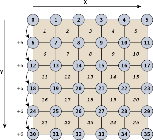
So if we want to find the number of the first point of a surface, we first have to calculate the start number of the row (y * size_x) and then add the X-position of the point (+ x). The next point of the surface is right next to it. So you only have to add 1 to the previous number (y * size_x + x + 1). The third point is one row lower (y + 1). Therefore its number is (y + 1) * size_x + x + 1. The fourth point is in the same row before the third point. So we have to subtract 1 again from the number of the third point ((y + 1) * size_x + x). If we repeat this for all surfaces, we get the desired list of parabola_surfaces.
For the surfaces of the base we can proceed in a similar way:
module parabola( focus_point, base_area, resolution = [10, 10] ){

    /* ... */

    size_x = resolution.x + 1;

    /* ... */

    size_ppoints = len( parabola_points );

    base_faces = [
        for (
            y = [0 : resolution.y - 1],
            x = [0 : resolution.x - 1]
        )
        [ y    * size_x + x     + size_ppoints,
          y    * size_x + x + 1 + size_ppoints,
         (y+1) * size_x + x + 1 + size_ppoints,
         (y+1) * size_x + x     + size_ppoints]
    ];

}
/* ... */
Since we will later append the base_points to the parabola_points, the numbers of the base points will shift by the number of parabola points. This shift is achieved by adding size_ppoints. Otherwise, nothing changes in the determination of the surfaces.
We have now defined the surfaces of the parabola and the base. What is still missing are the surfaces of the sides. Let’s start with one side:
module parabola( focus_point, base_area, resolution = [10, 10] ){

    /* ... */

    size_x = resolution.x + 1;

    /* ... */

    size_ppoints = len( parabola_points );

    /* ... */

    side_faces_1 = [
        for ( x = [0 : resolution.x - 1] )
        [ x,
          x + 1,
          x + 1 + size_ppoints,
          x     + size_ppoints ]
    ];

}
/* ... */
For the first side we run only once along the X-direction and connect the points from the array parabola_points with their corresponding points from the array base_points in pairs. Since the numbers of the base_points start at size_ppoints, we find the corresponding additions at points 3 and 4 of the surface.
The opposite side can be described in a similar way. Here we need to shift the numbers so that we do not run along the first row, but along the last row:
module parabola( focus_point, base_area, resolution = [10, 10] ){

    /* ... */

    size_x = resolution.x + 1;

    /* ... */

    size_ppoints = len( parabola_points );

    /* ... */

    last_row = resolution.y * size_x;

    side_faces_2 = [
        for ( x = [0 : resolution.x - 1] )
        [
            last_row + x,
            last_row + x + 1,
            last_row + x + 1 + size_ppoints,
            last_row + x     + size_ppoints
        ]
    ];

}
/* ... */
We achieve this by calculating the starting number of the last row (last_row = resolution.y * size_x;) and adding it at each point of the surface. Otherwise, everything remains the same as for side surface 1.
Now we come to the other two side faces. For these we do not have to run along the outer rows, but along the outer columns:
module parabola( focus_point, base_area, resolution = [10, 10] ){

    /* ... */

    size_x = resolution.x + 1;

    /* ... */

    size_ppoints = len( parabola_points );

    /* ... */

    side_faces_3 = [
        for ( y = [0 : resolution.y - 1] )
        [
            y      * size_x,
           (y + 1) * size_x,
           (y + 1) * size_x + size_ppoints,
            y      * size_x + size_ppoints
        ]
    ];

    last_col = resolution.x;

    side_faces_4 = [
        for ( y = [0 : resolution.y - 1] )
        [
            last_col +  y      * size_x,
            last_col + (y + 1) * size_x,
            last_col + (y + 1) * size_x + size_ppoints,
            last_col +  y      * size_x + size_ppoints
        ]
    ];

}
/* ... */
Overall, we see the same scheme for side faces 3 and 4 as for side faces 1 and 2. Side face 4 differs from side face 3 only in that we have shifted the numbers by the starting number of the last column. While the numbers of the points along the X-direction have the distance 1, the numbers of the points along the Y-direction have the distance size_x.
Groking the logic of the numbering of the points is not easy, especially in the beginning. It helps a lot to sketch the geometry on a sheet of paper and to label it with the numbers of the points. Just as it can be seen in figure 11..
Now we have finally gathered enough information to create our geometry with the basic shape polyhedron:
module parabola( focus_point, base_area, resolution = [10, 10] ){

    /* ... */

    polyhedron(
        points = concat( parabola_points, base_points ),
        faces  = concat( parabola_faces,
                         base_faces,
                         side_faces_1,
                         side_faces_2,
                         side_faces_3,
                         side_faces_4)
    );

}
/* ... */
We use the concat function to concatenate our point and surface sets and pass them as parameters points and faces to the 3D base shape polyhedron. If we now run a preview (F5) we should finally be able to see our parabola.
There are certainly use cases where you don’t want the full body below the parabola. We can adjust our module parabola in one place to provide the possibility to create only the parabola surface itself with a given thickness:
module parabola(
    focus_point,
    base_area,
    resolution = [10, 10],
    thickness  = 0
){

    /* ... */

    base_points = [
        for (
            y = [0 : base_area.y / resolution.y : base_area.y + 0.1],
            x = [0 : base_area.x / resolution.x : base_area.x + 0.1]
        )
        let ( p = parabola_point( focus_point, [x,y,0] ) )
        if (thickness > 0)
            [x, y, p.z - thickness]
        else
            [x, y, 0]
    ];

    /* ... */

}
/* ... */
For this extension we give our module parabola another parameter thickness, which gets the default value 0. Inside the module we change the calculation of the base points slightly. By means of let we calculate the current parabola point again and keep it in the variable p. Subsequently, we carry out a case distinction. If the parameter thickness is greater than zero, then we create a base point that is exactly thickness away from the parabola point p. Otherwise, if thickness is equal to 0, we create the base point as usual on the X-Y plane.
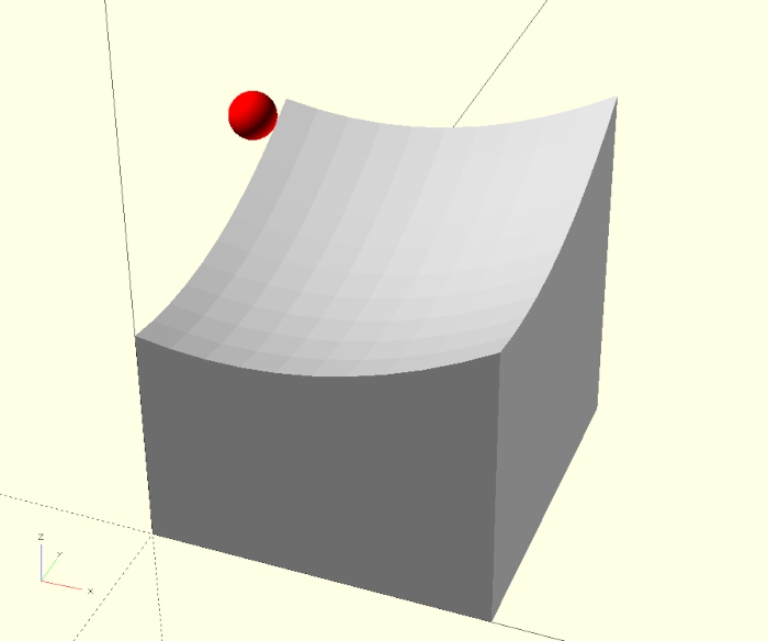
With this change, we can now create pure parabolic surfaces without a substructure (Figure 11.).
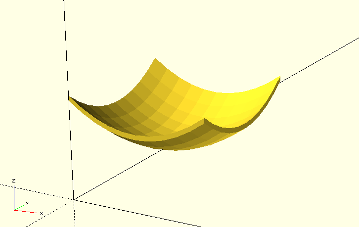
The basic 3D shape polyhedron is certainly not the first choice when you want to describe a 3D geometry with OpenSCAD. Using polyhedron requires some planning and is not free of subtle problems. For example, surfaces may not be displayed correctly. This generally has two possible causes. If the display errors only occur in the preview (F5), but not in the actual render (F6), then increasing the convexity parameter of the basic 3D shape polyhedron can help. By default this parameter has the value 1.
The second cause of errors is a bit more troublesome to fix. This is because the surfaces you have defined are only visible from one direction. If you would look from the inside of the object to the outside, you could see through the surfaces. Which side of the surfaces is visible and which is not depends on the order of the points with which we build up a surface. So a surface with the points [0, 1, 2, 3] or the points [3, 2, 1, 0] differs in whether the front or the back side is visible. A good tool to deal with such problems is to define a function flip which flips the order of the elements in a four-dimensional vector:
function flip(vec) = [ vec[3], vec[2], vec[1], vec[0] ];If the rendering of a set of surfaces is not ok, one can bring the function flip to bear on the definition of the surfaces and see if this solves the problem. This would look like this, for example:
    side_faces_1 = [
        for ( x = [0 : resolution.x - 1] )
        flip ([
            x,
            x + 1,
            x + 1 + size_ppoints,
            x     + size_ppoints
        ])
    ];
All in all, you will probably use polyhedron rather rarely. However, it represents a powerful tool with which one can solve difficult modeling tasks.
The further the focal point is away from the parabolic surface, the flatter the surface will become. In such a case, try to print the parabolic surface vertically. This will make the surface of the parabola finer, as 3D printers usually have a higher resolution in the X-Y plane than in the Z-axis.
If you need a parabola with a different outer shape, e.g. round, you can easily achieve such a shape by using the Boolean operation intersection with, e.g., a cylinder.