
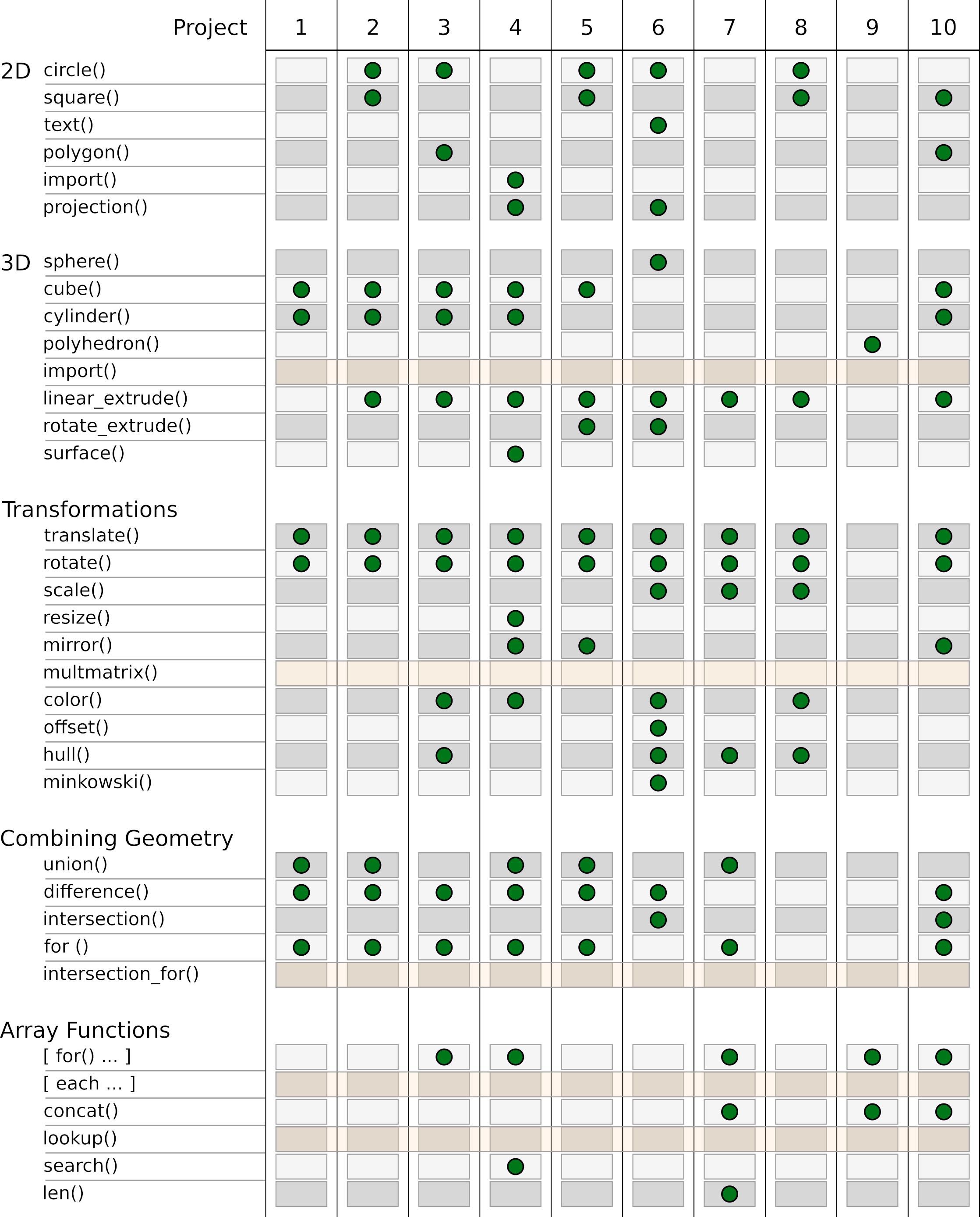
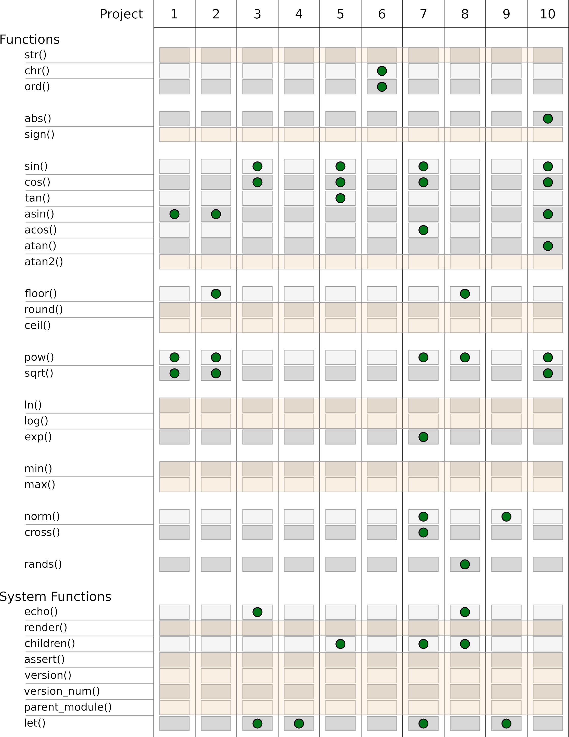
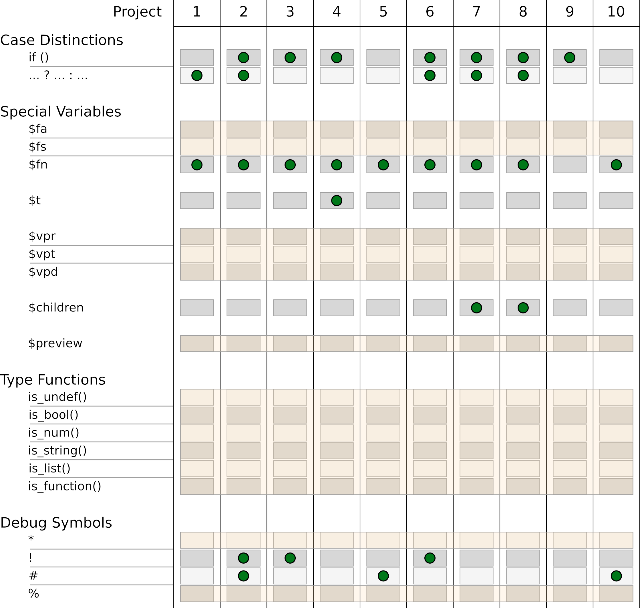
In the past 10 projects we got to know almost the entire range of functions in OpenSCAD. Figures 13., 13.2 and 13.3 provide an overview of this. In the following we will briefly discuss the functions that we have left out so far.
In project 4, we used the import function to import .svg files as a 2D basic shape. However, the import function can also import 3D data in .stl, .off, .amf and .3mf formats. Especially if you want to use a complex and computationally intensive OpenSCAD geometry in another project, using import instead of include or use can be useful. This way you avoid in many cases a recalculation of the complex geometry. The disadvantage is, of course, that you can no longer parameterize the imported geometry directly.
The only transformation we have not used is the multmatrix transformation. It allows to perform an affine transformation of the geometry via a transformation matrix. The matrix is a 4 x 3 or 4 x 4 matrix whose cells have the following meaning:
M = [
	// the first row is concerned with X
	[
		1, // scaling in X-direction
	  	0, // shear of X along Y
	  	0, // shear of X along Z
	  	0, // translation along X
	],

	// the second row is concerned with Y
	[
		0, // shear of Y along X
	  	1, // scaling in Y-direction
	  	0, // shear of Y along Z
	  	0, // translation along Y
	],

	// the third row is concerned with Z
	[
		0, // shear of Z along X
	  	0, // shear of Z along Y
	  	0, // scaling in Z-direction
	  	0, // translation along Z
	],

	// the fourth row is always:
	[0, 0, 0, 1]

];

multmatrix(M)
cube([10,10,10]);
Since the fourth row of the matrix M is fixed, it can also be omitted when using multmatrix. With the appropriate assignment of the entries of matrix M one can perform any translations or rotations and combine them by matrix multiplication. In practice, multmatrix is rarely used. Only the possibility to shear an object in a certain direction is sometimes useful.
We have used for-loops in many places in the 10 projects. The resulting geometries are implicitly combined as a Boolean union. This can be seen well in the following example:
module test() {

    echo($children);

    children();

}

test() {
    sphere(5);

    translate( [10, 0, 0] )
    sphere(5);

    translate( [20, 0, 0] )
    sphere(5);
}

test()
for(i = [0:2])
translate( [10 * i, 10, 0] )
sphere(5);
We define a module test, which outputs the number of elements of the subsequent geometry in the console window. If we use test with a geometry set ({ ... }) we get an output of 3 in the above example. If we use test with a for-loop, we get an output of 1. Thus, the geometries defined by the for-loop are combined into a single geometry. This means that it is not possible to describe a set of geometries with a for-loop and then apply the Boolean operation intersection on this set of geometries. Exactly for this case there is the intersection_for-loop in OpenSCAD. In practice, this type of for-loop is rarely used. But it can be used to create interesting geometries. This diamond-like geometry may serve as an example:
M = [
    [1,0,1,0],
    [0,1,0,0],
    [0,0,1,0]
];

intersection_for(i = [0:60:359])
rotate( [0, 0, i] )
multmatrix( M )
cube( 10, center = true );We have used generative for-loops in many places to define arrays. Within such a generative for-loop, the keyword each can be used to “unpack” a vector. Let’s look at the following example:
vectors = [
    [1,2,3],
    [4,5,6],
    [7,8,9]
];

flattened = [ for (v = vectors) each v];

echo( flattened );
The variable flattened is a one-dimensional array, which contains all entries of the two-dimensional array vectors. The console output for flattened therefore results in ECHO: [1, 2, 3, 4, 5, 6, 7, 8, 9].
The lookup function interpolates values in an array of number pairs to be linearly. An example:
values = [
    [-3,  2],
    [ 0, 10],
    [ 1, 50],
    [ 4,  0]
];

echo( lookup(-1,   values) );
echo( lookup( 0,   values) );
echo( lookup( 0.5, values) );
echo( lookup( 3,   values) );
The console output for this looks like this:
ECHO: 7.33333
ECHO: 10
ECHO: 30
ECHO: 16.6667
The lookup function searches the array of number pairs passed to it for the two adjacent number pairs whose first values span an interval in which the passed search parameter lies. Subsequently, the second values of these two pairs are averaged such that the resulting average corresponds to the proximity of the search parameter to the respective first values.
We have used a large part of the functions provided by OpenSCAD in our projects. We did not use the functions str, sign, atan2, round, ceil, ln, log, min and max.
The function str creates a single, contiguous string from its parameters. You remember the variable srnd from project 8? We used the variable for initializing random numbers and output its value to the console using echo( srnd ); to remember it for later, manual use. We could have made this console output a bit more readable with the str function, e.g. echo( str("As initialization value ", srnd, " was used.") );.
The function sign returns the sign of a number. For negative numbers sign returns a -1, for positive numbers a 1 and for zero a 0.
The function atan2 is a variant of the arc tangent. The “normal” arc tangent cannot distinguish between y/x and -y/-x, since the minus signs would cancel out in the second case. The function atan2 solves this problem by passing y and x as separate parameters to the function.
The round function rounds the passed decimal value commercially. The function ceil always rounds up the passed value.
The function ln returns the natural logarithm of the given number. The function log returns the logarithm to the base 10.
The function min returns as result the smallest value of the parameters passed to it. If the parameter consists of only one vector, the smallest element within the vector is returned. The function max behaves analogously. It returns the largest element in each case.
In rare cases it can happen that the preview (F5) of a geometry fails and artifacts occur which cannot be dealt with by other means (e.g. a convexity parameter). With the function render, which can be prepended to any geometry like a transformation (e.g. render() sphere( 10 );), one can force OpenSCAD to calculate the corresponding part of the geometry completely even during a preview.
Another use of render is to convert complex geometry into a 3D model already in the preview, thus making the preview smoother. This can be particularly helpful for complex Boolean operations.
The assert function facilitates checking of assumptions and allows to output an appropriate error message if these assumptions are not met. This is especially useful when we develop modules that are to be used by others as a library. Let’s assume we expect a three-dimensional vector as input. Then a check could look like this:
module my_module( size ) {

    assert(
        len(size) == 3,
        "Parameter size must be a three-dimensional vector!"
    );
}
If we would now call the module e.g. with a simple number, we would get an error message in the console:
ERROR: Assertion '(len(size) == 3)' failed: "Parameter size must be a three-dimensional vector!"The type checking functions described below can be very useful in this context.
The functions version and version_num return the current version of OpenSCAD. The version function returns a three-dimensional vector with the individual version components. The function version_num returns a single number uniquely representing the respective version.
Such a version query is useful when we develop a geometry library and use functions that are not available in earlier versions of OpenSCAD or have been parameterized differently. By appropriate case distinctions one can achieve it that the library remains stable over several versions of OpenSCAD.
The function parent_module returns the name of a parent module within a module hierarchy, if all modules within the hierarchy access child elements by means of children. The official manual of OpenSCAD gives the generation of a material list as an application example. In practice, this function does not play any role.
In our projects we often used the special variable $fn to set the level of detail of curved geometries. In a similar way, the level of detail of curved geometries can also be controlled using the variables $fa and $fs. With $fa you can set the minimum angles of a geometry and with $fs the minimum size of the individual surfaces. In both cases, smaller values result in a finer geometry. By default $fa is set to 12 and $fs to 2.
The special variables $vpr, $vpt and $vpd provide information about the current perspective in the output window when a new preview is rendered. $vpr provides the rotation, $vpt the displacement and $vpd the distance of the camera.
By setting these variables you can change the perspective in the output window. This could be used, for example, to create tracking shots in connection with the animation capabilities of OpenSCAD.
The special variable $preview returns true if a preview (F5) is run and false if a full geometry render (F6) is performed.
OpenSCAD provides a number of functions that can be used to check the type of a variable. This check is especially useful in connection with the assert function, or in case you want to provide a parameter with double functionality. An existing example of this is the scale parameter of the linear_extrude transformation. The parameter can be either a number or a vector. If it is a number, the underlying 2D shape is scaled equally in all directions. If the parameter is a vector, individual scaling can be specified for the X- and Y-directions.
The available type functions are: is_undef, is_bool, is_num, is_string, is_list and (in future OpenSCAD versions) is_function. With list any kind of arrays or vectors are meant.
Besides the known debug characters ! and # there is also the * character and the % character. With the * character you can “disable” a geometry part. It is an alternative to commenting it out. With the % character you can make a geometry part transparent.
With this final short summary you now know all OpenSCAD functions!