
In this project we construct a shelf bracket. Both the lengths of the two sides and the size and number of the holes will be freely adjustable.
We will learn about union as a new Boolean operation. In addition, we will use a few mathematical functions (root, power and arc cosine) from OpenSCAD and learn more about modules. Last but not least, we will look at the projection function as we use it to create drilling templates for our shelf bracket.
To start, let’s create an empty module shelf_bracket and think about what parameters we need. We want to be able to change the length of each side, as well as the size and number of holes. In addition, our bracket will have a width and we need to know what material thickness the bracket should have. That’s a lot of parameters! To keep our parameter list short, we can combine the values of each side (length, hole diameter, number of holes) into a three-dimensional vector:
/*
	module shelf_bracket

	parameters:
	- side_a    is a vector [length, hole diameter, number of holes]
	- side_b    is a vector [length, hole diameter, number of holes]
	- width     refers to the width of the bracket
	- thickness refers to the material thickness of the bracket
 */

module shelf_bracket( side_a, side_b, width, thickness ) {

}

shelf_bracket(
  side_a    = [50, 6, 1],
  side_b    = [75, 4, 3],
  width     = 35,
  thickness = 4
);
Above our module we have written a multiline comment (/* ... */) that briefly explains what parameters there are and what kind of input these parameters expect. Even if nobody else will use your module, such a comment is useful. If you need a shelf bracket again in 6 months, you will be glad about the helpful comment! Below the module shelf_bracket we have instantiated the module once with concrete values. Without this instance, we would not see any geometry in the output window as we develop our module step by step. In addition, we can use the instance to change the parameters every now and then during development to check whether our geometry description behaves as expected.
If you look at the shelf bracket in figure 3., you will notice that the two sides of the bracket are basically the same. They consist of a plate and evenly distributed holes along the central axis. We need this geometry for both sides. Therefore, it is worth encapsulating one side within a module and use it twice. Since we need this module only for the bracket, we define it inside the module shelf_bracket as submodule xhole_plate and then use the submodule for side A and side B of the bracket:
/* ... */
module shelf_bracket( side_a, side_b, width, thickness, ) {

	module xhole_plate(size, h_dm, h_num, margin) {

		difference(){

			cube(size);

			h_distance = (size.x - margin) / (h_num + 1);

		    for (x = [1:h_num])
		    translate ([
		        margin + x * h_distance,
		        size.y/2,
		        -1
		    ]) cylinder( d = h_dm, h = size.z + 2, $fn=18);

		}
	}

	// side A
	xhole_plate(
		[side_a[0], width, thickness],
		side_a[1],
		side_a[2],
		thickness
	);

	// side B
    translate([thickness,0,0])
    rotate([0,-90,0])
	xhole_plate(
		[side_b[0], width, thickness],
		side_b[1],
		side_b[2],
		thickness
	);

}

/* ... */
The submodule xhole_plate gets as parameters the size of the side part as a three-dimensional vector (size), the diameter (h_dm) and the number (h_num) of the holes as well as a margin. The latter is needed as the surface area of the sides is reduced by the thickness of the material at the point where the two sides of the bracket meet. Since we want to distribute our holes along this surface, we have to take this reduction into account. Theoretically, we could have derived the material thickness from the parameter size (size.z). The use of an extra parameter simply makes it easier to read and understand.
We model the plate with a simple cube, passing it the size parameter (cube(size);). We create the holes with a for-loop and then subtract them from the plate using the Boolean difference operation. In this example we let the for-loop run from 1 to the number of holes (x = [1:h_num]) and calculate the actual position of the respective hole directly in the translate transformation inside the loop (margin + x * h_distance). We always start with the margin and then add the appropriate number of hole distances. We have defined the hole distance (h_distance) before the loop. For this we divided the available length (length of the side minus margin) by the number of hole interspaces (number of holes plus 1). For the holes themselves, we use a cylinder to which we assign the parameter h_dm as the diameter d. We determine the height h from the height of the plate (size.z) and two millimeters allowance, so that our hole will be clean. Matching this allowance, we put a value of -1 (i.e. half the allowance) as z-shift in the translate transformation. As a result, the cylinder protrudes exactly 1 millimeter above and below the plate. The third parameter $fn=18 of the cylinder is new. It is a “special variable” of OpenSCAD with which you can set the level of detail of curved geometries. The larger the value of $fn is, the finer the geometry becomes. Though, keep in mind that values of more than 100 for the variable $fn are practically never needed and would only make the geometry unnecessarily complex. You can also set the variable $fn “globally”. In this case it influences all curved geometries of your model. However, experience shows that it is better to use it specifically where you want to increase the level of detail instead of increasing the level of detail everywhere.
Directly below the module definition of xhole_plate we use the module for the two sides A and B. Since side B is perpendicular to side A, we need to rotate it by 90 degrees. In this specific case it is minus 90 degrees, because we want to rotate counterclockwise around the Y-axis. After the rotation, the position of side B is still not quite right. We have to move it by the material thickness along the X axis. Otherwise, side A would become too long.
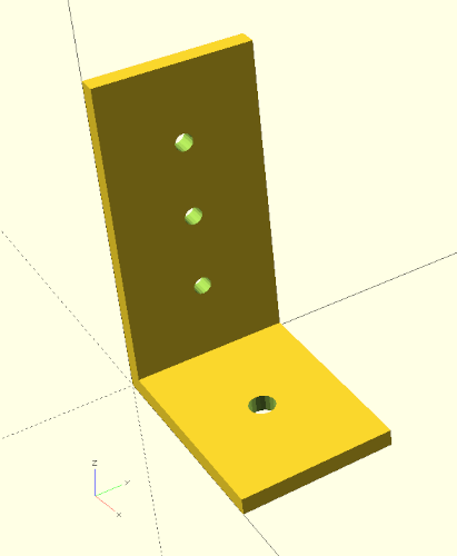
Our shelf bracket already looks pretty acceptable by now (Figure 3.) and changing the parameters demonstrates that our geometry description behaves as expected. What we are still missing are two stringers to make our bracket more stable. We first create the stringers from two boxes (cube), which we define below sides A and B in our module shelf_bracket:
/* ... */
module shelf_bracket( side_a, side_b, width, thickness ) {

	module xhole_plate(size, h_dm, h_num, margin) {
		/* ... */
	}

	// side A
	xhole_plate(
		[side_a[0], width, thickness],
		side_a[1],
		side_a[2],
		thickness
	);

	// side B
    translate([thickness,0,0])
    rotate([0,-90,0])
	xhole_plate(
		[side_b[0], width, thickness],
		side_b[1],
		side_b[2],
		thickness
	);

	// stringer
	cube( [side_a[0], thickness, side_b[0]] );

	translate( [0, width - thickness, 0] )
	cube( [side_a[0], thickness, side_b[0]] );

}

/* ... */
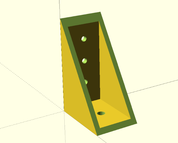
From a purely technical point of view, our stringers already serve their purpose (Figure 3.). However, it would be nicer if our shelf bracket had tapered stringers. We can achieve this by subtracting a suitably rotated box from our existing bracket. To make this possible, we need to combine our previous geometry description, which consists of four individual geometries (two times xhole_plates and two cubes) into a single geometry. This can be done using the Boolean union operation:
/* ... */
module shelf_bracket( side_a, side_b, width, thickness ) {

	module xhole_plate(size, h_dm, h_num, margin) {
		/* ... */
	}

	union() {

		// side A
		xhole_plate(
			[side_a[0], width, thickness],
			side_a[1],
			side_a[2],
			thickness
		);

		// side B
	    translate([thickness,0,0])
	    rotate([0,-90,0])
		xhole_plate(
			[side_b[0], width, thickness],
			side_b[1],
			side_b[2],
			thickness
		);

		// stringer
		cube( [side_a[0], thickness, side_b[0]] );

		translate( [0, width - thickness, 0] )
		cube( [side_a[0], thickness, side_b[0]] );

	}

}

/* ... */
Like with the Boolean difference operation, we combine the individual geometries by surrounding them with a set of curly brackets ({ ... }). Instead of the keyword difference, we now use the keyword union. Having combined our four geometries this way we can now subtract a rotated box to create the desired taper of the stringers.
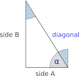
We now need to know how big this rotated box must be and at what angle it must be tilted (Figure 3.). Here vague memories of math lessons can help us. According to Pythagoras the sum of the squares of the sides is equal to the square of the main side in a right triangle. So if you take the square root of the sum of the side squares, you get the length of the diagonal you are looking for. The angle can be determined by the arc cosine. As you can look up on, e.g., Wikipedia, the cosine of an angle is equal to the adjacent divided by the hypotenuse. Here, the hypotenuse is our diagonal, and the adjacent is the side against which the angle lies (as opposed to the opposite, which lies opposite to the angle). We can calculate both values, the length of the diagonal and the angle of the diagonal, with the mathematical functions provided by OpenSCAD and then use them for the correct positioning and rotation of the box:
/* ... */
module shelf_bracket( side_a, side_b, width, thickness ) {

	module xhole_plate(size, h_dm, h_num, margin) {
		/* ... */
	}

	difference() {

		union() {

			// side A
			xhole_plate(
				[side_a[0], width, thickness],
				side_a[1],
				side_a[2],
				thickness
			);

			// side B
		    translate([thickness,0,0])
		    rotate([0,-90,0])
			xhole_plate(
				[side_b[0], width, thickness],
				side_b[1],
				side_b[2],
				thickness
			);

			// stringer
			cube( [side_a[0], thickness, side_b[0]] );

			translate( [0, width - thickness, 0] )
			cube( [side_a[0], thickness, side_b[0]] );

		}

		diag  = sqrt( pow(side_a[0], 2) + pow(side_b[0], 2) );
		angle = asin( side_a[0] / diag );

		translate( [side_a[0], -1, 0] )
		rotate( [0, -angle, 0] )
		cube( [diag, width + 2, diag + 2] );

	}

}

/* ... */
Below the geometry set of the union operation we first calculate our diagonal and our angle. The function sqrt calculates the square root and the function pow calculates the power of a number. For the power function the first parameter is the number (here: side_a[0] or side_b[0]) you want to exponentiate and the second parameter is the exponent (here: 2). We calculate the angle with the help of the arc cosine (acos) as described above from the quotient of the adjacent and the hypotenuse (here: side_a[0] divided by diag). Subsequently we create a box (cube) which is diag long, width + 2 wide and diag + 2 high. Again, we added some small allowance of two millimeters to both width and height so that our difference operation will perform cleanly later. We rotate the box around the Y axis counterclockwise (hence the -). As angle we do not use the angle we calculated directly, but 90 degrees minus the angle. This is because we actually need the angle that is shaded blue in Figure 3.. If you remember your math class particularly well, you might now argue that we should have taken the arc sine right then, since it provides the alternate angle of the angle we need. And you would be right!
After we have rotated our box, all we have to do is move it to the correct position. This is done with a translate transformation. As expected, we shift our box by the length of side A along the X-axis. The shift of -1 along the Y-axis serves to ensure a clean difference operation and matches the allowance of 2 millimeters in width. We do not need to worry about the addition in height at this point, since it is sufficient if the box overhangs our bracket in the tilting direction.
Now that the box is in the right position, we can finally subtract it from our bracket geometry. To do this, we enclose the union we created earlier and the box we just created in a pair of curly brackets again ({ ... }) and prepend the Boolean difference operation to the whole thing. Done!
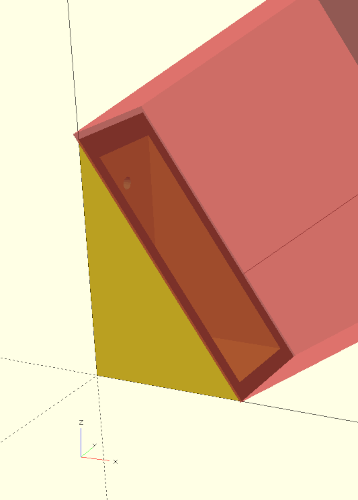
#A hint: if we want to check the position of our box without having to detach it from the Boolean difference operation, we can temporarily prepend a # to the box (cube). If we now run a preview, the box will be displayed in a semi-transparent color (Figure 3.).
Let’s assume we have printed our shelf bracket with a 3D printer and now want to mount it onto the wall. Wouldn’t it be handy if we now had a drilling template? We can create such a template by using a 3D to 2D projection, which is available in OpenSCAD via the projection transform:
/* ... */

projection(cut = true)
shelf_bracket(
  side_a    = [50, 6, 1],
  side_b    = [75, 4, 3],
  width     = 35,
  thickness = 4
);
The projection transform acts like every transformation on the following element and projects it onto the X-Y plane. This results in something like the two-dimensional shadow of the geometry. If you pass the parameter cut = true to the projection transform (as we do here), then the geometry is cut in the X-Y plane and only the cut is displayed. In the case of our shelf bracket, both variants lead to the same result. By the way, in order for the section to really be displayed as 2D geometry, you have to trigger a full rendering (F6) of the geometry and not just a preview (F5). After rendering (F6) the 2D geometry can be exported as SVG (File -> Export -> Export as SVG) and printed with a graphics program like Inkscape.
If we now also want to have a drilling template of side B, we must rotate our bracket by 90 degrees counterclockwise around the Y axis:
/* ... */

projection(cut = true)
rotate( [0, -90, 0] )
shelf_bracket(
  side_a    = [50, 6, 1],
  side_b    = [75, 4, 3],
  width     = 35,
  thickness = 4
);
We could leave it at that and comment the lines with the projection and rotation in and out as needed. Alternatively, we can define a special module that can switch between 3D geometry and drilling templates on demand:
/* ... */
module output(templates = false) {
if (templates) {
projection(cut = true)
children(0);
translate( [-0.01, 0, 0] )
projection(cut = true)
rotate( [0, -90, 0] )
children(0);
} else {
children(0);
}
}
output(templates = false)
shelf_bracket(
side_a = [50, 6, 1],
side_b = [75, 4, 3],
width = 35,
thickness = 4
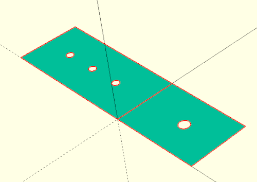
);The module output has a parameter templates. If it is set to true, then the drilling templates of sides A and B will be created (Figure 3.). If the parameter is set to false, the normal 3D geometry is generated. Within the module output we switch between these two modes by using an if-statement. The expression if (templates) is an abbreviation of if (templates == true). But how does our shelf bracket geometry get into the module output? This is done by the keyword children. With it we get access to the element following our module! The parameter 0 indicates that we want to have the first element. If our module would be followed by a geometry set enclosed in curly brackets ({ ... }), we could also access further elements. In this case, the special variable $children would tell us how many elements there are. In our case, however, we know that there is only one subsequent element (our shelf bracket). Thus, we do not need $children at this point.
In general, the children keyword allows us to define modules that behave like transformations. For the most time, one does not need this capability too often. However, there are situations where it can be used to achieve very elegant solutions for otherwise elaborate geometry descriptions.
If we want to print our geometry with a 3D printer, we have to render our geometry first (F6). Depending on the complexity of the geometry, this can sometimes take a few minutes. Just be patient here. When the rendering is done, you can export the resulting geometry (File -> Export -> Export as …). A typical format is .stl. You can then load the .stl file into a so-called slicer software and prepare the geometry for 3D printing.
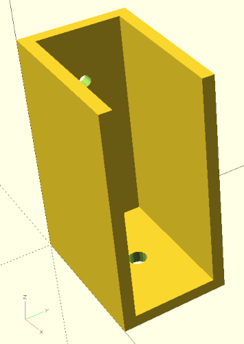
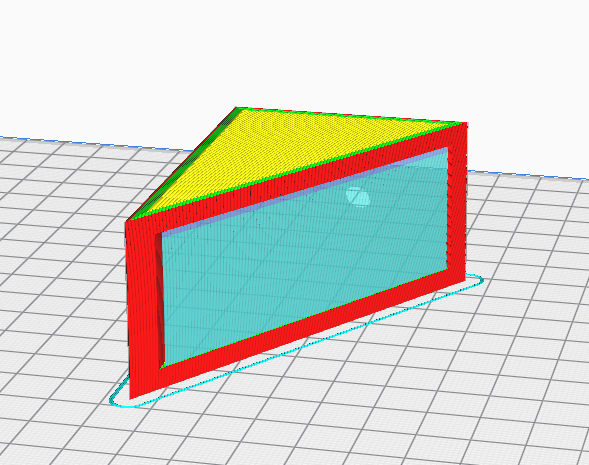
Within the slicer software, the question arises in which orientation one would like to print the shelf bracket. Since 3D-printed components are created in layers, the stability of the components within a layer is significantly greater than between the layers. In particular, shear forces acting on the layers can cause a component to break. For our shelf bracket, it would therefore be best to print it lying on its side. One disadvantage of this orientation is that you need a support structure within the component to stabilize the top-lying stringer during printing (Figure 3.).
An alternative orientation, which may not require a support structure but still results in a stable part, is to print the bracket lying on the tapered side. Finding the right angle for this orientation directly in the slicer software can be a bit tricky. In this case it is easier to export the geometry already in the correct orientation from OpenSCAD. We can extend our module shelf_bracket once again to support this orientation:
module shelf_bracket( side_a, side_b, width, thickness, rotate_it = false ) {

	module xhole_plate(size, h_dm, h_num, margin) {
		/* ... */
	}

	diag  = sqrt( pow(side_a[0], 2) + pow(side_b[0], 2) );
	angle = asin( side_a[0] / diag );

	rotate( [0, rotate_it ? 90 + angle : 0, 0] )
	difference() {

		union() {

			// side A
			xhole_plate(
				[side_a[0], width, thickness],
				side_a[1],
				side_a[2],
				thickness
			);

			// side B
		    translate([thickness,0,0])
		    rotate([0,-90,0])
			xhole_plate(
				[side_b[0], width, thickness],
				side_b[1],
				side_b[2],
				thickness
			);

			// stringer
			cube( [side_a[0], thickness, side_b[0]] );

			translate( [0, width - thickness, 0] )
			cube( [side_a[0], thickness, side_b[0]] );

		}

	    translate( [side_a[0], -1, 0] )
	    rotate( [0, -angle, 0] )
	    cube( [diag, width + 2, diag + 2] );

	}

}
We add to our module another parameter rotate_it and give it the default value false. Then we move the calculation of the diagonal and the angle upwards in front of the Boolean difference and rotate the whole object around the Y-axis clockwise by ‘90 + angle’ degrees if the parameter rotate_it is true. Otherwise we do not rotate (0 degrees).
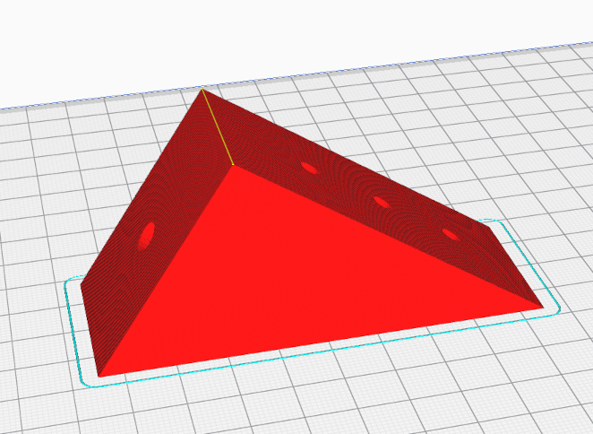
If we now export our geometry again as .stl file, our part lies in the correct orientation for the slicer software and can be printed without a support structure but still as a strong object (Figure 3.).
After you have printed the shelf bracket, it is advisable to measure all the dimensions of the printed object once. In particular, the holes may not have been printed true to size. If this is the case, you can now benefit from the power of parametric modeling. You can simply adjust the diameters accordingly in the shelf bracket parameters and have an adjusted geometry generated at the push of a button.