
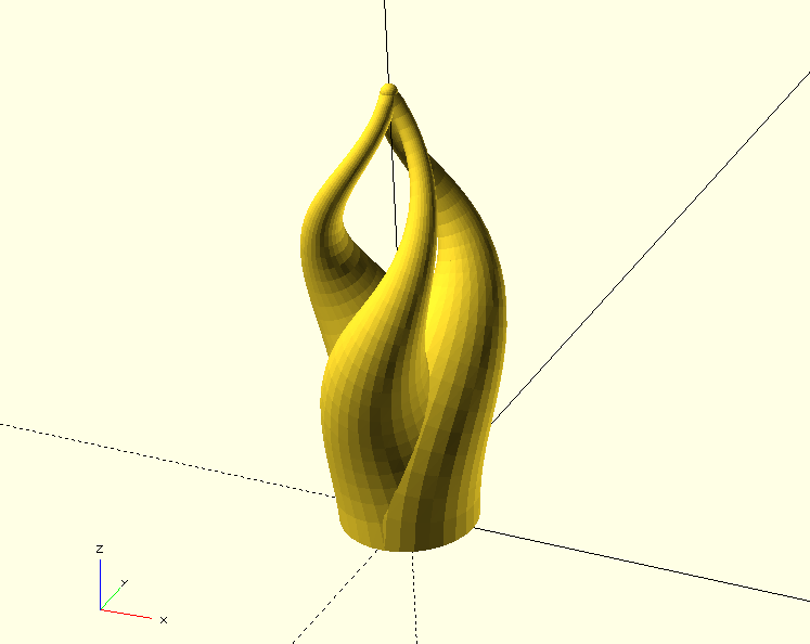
In the majority of cases, OpenSCAD is used for the design and geometric description of technical systems or components. However, this does not mean that organic shapes could not also be created with OpenSCAD. In this project we will create a flame sculpture that we will model using a number of mathematical functions.
In this project we will learn more about mathematical functions available in OpenSCAD (exp, norm, cross) and we will also create our own functions. In this context we will define a recursive function for the first time. Furthermore we will see how we can cascade the children call over several module levels and learn what the concat command is all about.
Let’s start with the module description and test instance of our module. Unlike with the previous projects, we will define all parameters right at the beginning and not introduce them bit by bit:
// Eine Flammenskulptur

module flames(
    height,
    scaling_start     = [1.0, 1.0, 1.0],
    scaling_end       = [0.1, 0.1, 0.1],
    x_radius          = 15,
    y_radius          = 10,
    steepness         = 0.2,
    transition        = 0.35,
    height_distortion = 0.7,
    turns             = 1,
    slices            = 30
) {


}

flames(180) {
    circle( d = 60 , $fn = 30);
    sphere( d = 60 );
}
If you look at the test instance of our module flames below the module description, you will see that the module will operate on a geometry set. Doing so allows us to subsequently change the underlying geometries and thus modify the character of our sculpture.
The basic idea for our model is to first compute a set of positions describing a curved path and then move a 2D basic shape along this path and transform it into a 3D geometry by using the hull transformation in a pairwise fashion. In addition, the underlying 2D basic shape will be scaled along the path. Let’s start with the generation of the curved path:
module flames(
height,
scaling_start = [1.0, 1.0, 1.0],
scaling_end = [0.1, 0.1, 0.1],
x_radius = 15,
y_radius = 10,
steepness = 0.2,
transition = 0.35,
height_distortion = 0.7,
turns = 1,
slices = 30
) {
// positions along the path
increment = height / slices;
rot_inc = 360 * turns / slices;
positions = [ for (i = [0:slices]) [
cos( i * rot_inc) * x_radius,
sin( i * rot_inc) * y_radius,
pow( i / slices, height_distortion) * height
]];
}
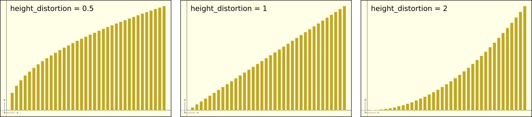
/* ... */The parameter height specifies the height of the path we want to create. The parameter slices specifies the number of steps we want to calculate along the path. From this we can determine an increment as an internal variable, which we will need later. Analogously, we derive a rotation increment rot_inc. We store the positions along our path as three-dimensional vectors within an array. We compute the array using a generative for-loop. Here, the X- and Y-coordinates of our positions move along an elliptical circular path with radii x_radius and y_radius while the Z-coordinate moves upwards. Instead of letting the Z-coordinate grow linearly, we use a power function to be able to influence the distribution of points along the Z-axis with the parameter height_distortion. Figure 9. gives an impression of how the power function behaves for different values of the parameter height_distortion.
Besides positioning, we also want to scale our basic shape along the path. Instead of scaling linearly we will use a sigmoid function. Since OpenSCAD does not offer a “ready-made” sigmoid function, we have to create one ourselves:
module flames(
height,
scaling_start = [1.0, 1.0, 1.0],
scaling_end = [0.1, 0.1, 0.1],
x_radius = 15,
y_radius = 10,
steepness = 0.2,
transition = 0.35,
height_distortion = 0.7,
turns = 1,
slices = 30
) {
// positions along the path
/* ... */
// scaling along the path
function sigmoid(x, steepness = 0.5, transition = 0.5) =
let (
increment = 1.0 - pow( steepness, 0.1),
starting_point = -transition / increment
) 1 / ( 1 + exp( -( x / increment + starting_point) ) );
s_factors = [ for (i = [0:slices])
1.0 - sigmoid( i / slices, steepness, transition )
];
}
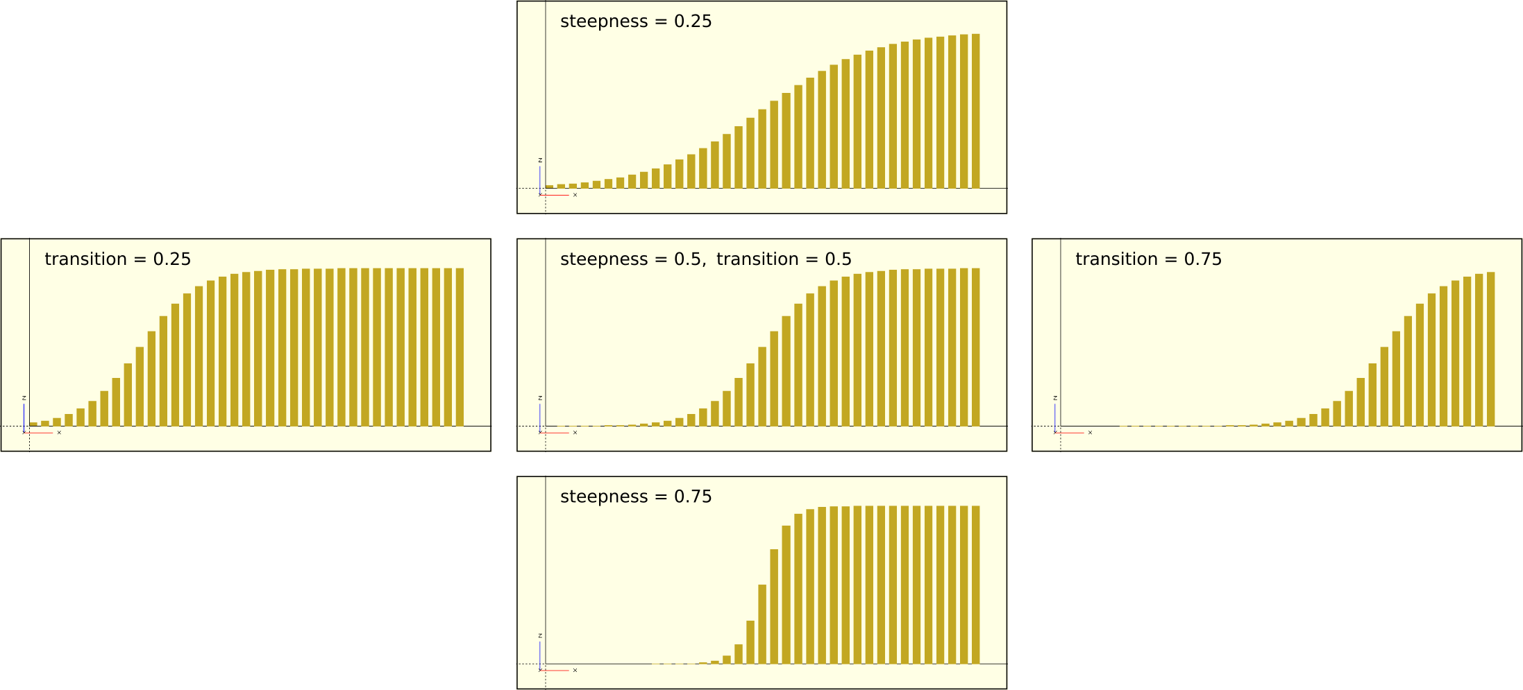
/* ... */We define our sigmoid function by means of the exponential function exp and the well-known scheme 1 / (1 + exp(-x) ). In addition, we parameterize our function in such a way that the sigmoidal transition lies in the interval 0 to 1 of the parameter x. Furthermore, we scale the function so that we can set the relative position and slope of the sigmoidal transition by means of the parameters steepness and transition. These two parameters also expect values between 0 and 1. Figure 9. gives an impression of the effect different values for steepness and transition have on the output of the function.
Like the positions, we calculate the scaling factors using a generative for-loop and store them in the s_factors array. Before we continue, let’s create a temporary version of a single flame to see if we are on the right track:
module flames(
    /* ... */
    scaling_start     = [1.0, 1.0, 1.0],
    scaling_end       = [0.1, 0.1, 0.1],
    /* ... */
) {

    // positions along the path
    /* ... */


    // scaling along the path
    /* ... */

    // a single flame
    module flame() {

        for (i = [1:slices])
        translate( positions[i] )
        linear_extrude( height = 2 )
        scale(
            scaling_start * s_factors[i] +
            scaling_end * (1.0 - s_factors[i])
        )
        children(0);

    }

    flame() children(0); // debug

}

flames( 180 ) {
    circle( d = 60 , $fn = 30);
    sphere( d = 60 );
}
We define a submodule flame and inside this module we use a single for-loop to go through the positions array and the s_factors array in parallel and use their values to scale and translate the 2D geometry. We create the actual scaling vector as a linear interpolation between scaling_start and scaling_end, taking the interpolation ratio from the s_factors array.
Between scaling and translation we perform a linear extrusion to transform the 2D geometry into a 3D geometry. As 2D geometry, we use children(0), i.e. the element that follows the instance of the submodule flame. Below the definition of the submodule flame we have instantiated a test instance of the module. As subsequent element we have used children(0) again! This children(0) refers now to the element that follows the instance of the module flames (plural!). If we look at its instance, we see that here the first subsequent element is a circle with a diameter of 60. The chain of calls to children() forwards this outer element down into the submodule flame.
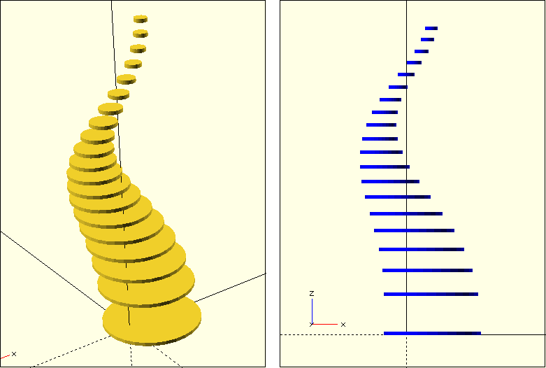
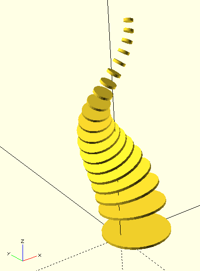
Figure 9. shows our intermediate result so far. The circle geometry recognizably follows a curved path and is scaled in the process. Theoretically, we could now connect the circles pairwise using the hull transformation and would obtain an already quite passable 3D geometry. However, it would be much nicer if the circles would tilt according to the local orientation of the path. To implement this, we need to figure out in which direction the path points at each position and then rotate the circle to match that direction. To figure that out we need some mathematics.
We get the cosine of the angle between two vectors if we divide the dot product of the two vectors by the product of the lengths of the two vectors. For the calculation of the length of a vector OpenSCAD offers the function norm. The calculation of the dot product we have to define ourselves. The dot product of two vectors v1 and v2 is calculated by multiplying the individual components of the vectors together and then summing up these products (v1[0] * v2[0] + v1[1] * v2[1] + ... + v1[n] * v2[n]). In most programming languages, we would go through the vectors one element at a time to do this, and gradually build our sum. In OpenSCAD we cannot create such a “running sum”, because variables can only be assigned once. A solution to this problem is the use of recursion:
module flames(
    /* ... */
) {

    // positions along the path
    /* ... */


    // scaling along the path
    /* ... */


    // angles along the path
    function dot_p(v1, v2, idx) =
        v1[idx] * v2[idx] + (idx > 0 ? dot_p(v1, v2, idx-1) : 0);

    function dot_product(v1, v2) = dot_p(v1, v2, len(v1)-1);


    // a single flame
    /* ... */

}
/* ... */
}
The function dot_p calculates the dot product of two vectors v1 and v2 in a recursive way. To do this the function needs a third parameter idx. The second function dot_product starts the recursion. It calls dot_p and sets at this initial call the value of the parameter idx to the index of the last element (len(v1) - 1) of the vectors. The function dot_p then calculates the product of the last elements of v1 and v2 and, depending on the value of idx, adds either a 0, or the value that the recursive call to the function dot_p yields. The key part - as with all recursive functions - is to make sure that the function does not call itself infinitely often. We achieve this here by giving the parameter idx the value idx - 1 when dot_p is called recursively. This way the value of idx becomes smaller with each recursive call. If it arrives at 0, no further recursive call takes place and the function is terminated. Along the way, we calculated the products of all elements and summed them up. The final result is the dot product of v1 and v2. If your head is buzzing a bit now: this is a normal side effect of dealing with recursive algorithms!
Now we can use our dot product to calculate the angles along the path:
module flames(
    /* ... */
) {

    // positions along the path
    /* ... */


    // scaling along the path
    /* ... */


    // angles along the path
    /* ... */

    function angle( v1, v2) = acos(dot_product(v1, v2) / (norm(v1) * norm(v2)));

    rel_pos = concat(
        [ positions[0] ],
        [ for (i = [1:slices]) positions[i] - positions[i-1] ]
    );

    pos_angles = concat(
        [0],
        [ for (i = [1:slices-1]) angle( [0,0,1], rel_pos[i]) ],
        [0]
    );


    // a single flame
    /* ... */

}
/* ... */
}
We first define the function angle, which gives us the angle between two vectors v1 and v2. As described before, we divide the dot product by the product of the lengths and determine the angle via the arc cosine function. To calculate the angles along the path, we first have to determine the relative directions of the individual path segments from our absolute positions. To do this, we create an array rel_pos that we combine from two arrays using the function concat. The first array contains only one element: the first position of our path. The second array contains for each following position of the path the difference between this position (positions[i]) and the previous position (positions[i-1]). Accordingly, the loop variable i does not start at 0 but at 1 (i = [1:levels]). Together, we get an array rel_pos whose entries go from 0 to slices. So it is as long as the array positions.
Now we have completed all preparations to finally be able to define the pos_angles array that will contain the angles along the path. Since we don’t want to rotate the first and the last 2D geometry, we compose the pos_angles array from three individual arrays. The first and last entries are simply set to 0. The entries in between are generated using a generative for-loop, which uses our function angle to calculate the angle between the vertical [0, 0, 1] and the respective relative path segment rel_pos[i]. Again, we made sure that the entries of the array pos_angles go from 0 to slices. This makes the later use of these arrays more elegant, as we can avoid some special case handling for the beginning and end of the path.
Now we can put the angle information to work in our temporary submodule flame:
module flames(
    /* ... */
) {

    // positions along the path
    /* ... */


    // scaling along the path
    /* ... */


    // angles along the path
    /* ... */

    // a single flame
    module flame() {

        for (i = [1:slices])
        translate( positions[i] )
        rotate( pos_angles[i], cross([0,0,1], rel_pos[i]) )
        linear_extrude( height = 2 )
        scale(
            scaling_start * s_factors[i] +
            scaling_end * (1.0 - s_factors[i])
        )
        children(0);

    }

    flame() children(0); // debug

}
/* ... */
}
We insert a rotate transform before the translation of the basic shape. We use the special variant of the rotate transform, to which we can separately pass an angle and a vector around which the rotation should take place. As angle we pass the previously determined angle from the field pos_angles. The rotation axis is the vector perpendicular to the vector of our relative direction rel_pos and the vertical ([0, 0, 1]). This vector can be calculated by the cross product of the other two vectors. Fortunately, we do not have to implement the cross product ourselves, but can use the OpenSCAD function cross instead. Figure 9. shows what our current intermediate result looks like.
In the next step, we need to modify the flame submodule a bit. After all, our goal is to connect the individual geometries along the path pairwise with the hull transformation. Therefore we detach the geometry description from the for-loop and move it into another submodule slice that we can index with the loop variable i:
module flames(
    /* ... */
) {

    // positions along the path
    /* ... */


    // scaling along the path
    /* ... */


    // angles along the path
    /* ... */

    // a single flame
    module flame() {

        module slice( i ) {
            translate( positions[i] )
            rotate( pos_angles[i], cross([0,0,1], rel_pos[i]) )
            linear_extrude( height = 0.01 )
            scale(
                scaling_start * s_factors[i] +
                scaling_end * (1.0 - s_factors[i])
            )
            children(0);
        }

        for (i = [1:slices])
        hull() {
            slice(i-1) children(0);
            slice(i) children(0);
        }

    }

    flame() children(0); // debug

}
/* ... */
}
The slice submodule encapsulates a single basic shape at the ith position along the path. Before, we used an extrusion length of 2 millimeters for our intermediate results. Now we reduce the extrusion length to 0.01 millimeters. This effectively brings us back to working with a 2D geometry, but allows us to manipulate it in 3D. The for-loop in the parent module flame connects the slices in pairs. Note that the loop variable i now starts from 1 instead of 0, so that we are allowed to make the statement slice(i-1) children(0); inside the geometry set of the hull transformation. As before, we need to pass the externally set geometry down into the slice submodule using children(0).
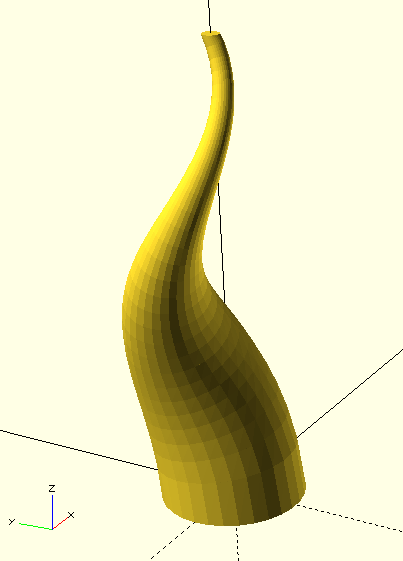
This completes the geometry description of a single flame (Figure 9.). What remains now is to arrange our single flame as a flame triplet. Before that, we should remove the test instance of the flame module (// debug):
module flames(
    /* ... */
) {

    // positions along the path
    /* ... */


    // scaling along the path
    /* ... */


    // angles along the path
    /* ... */


    // a single flame
    /* ... */


    // flame triplet
    translate([-x_radius,0,0])
    union(){
        flame()
        children(0);

        translate([x_radius,0,0])
        rotate([0,0,120])
        translate([-x_radius,0,0])
        flame()
        children(0);

        translate([x_radius,0,0])
        rotate([0,0,240])
        translate([-x_radius,0,0])
        flame()
        children(0);
    }

}
/* ... */
}
Our flame triplet consists of a Boolean union and three flames each rotated by 120 degrees relative to each other. Since the basic shapes inside the module flame always start their curved circular path at [x_radius, 0], we have to move the flames temporarily back to the origin before rotating them.
In its current form, the flame triplet ends up with a blunt tip. To improve the situation, we position a suitably scaled cap at the tip of the triplet. The geometry for this cap is supplied as the second element (children(1);) of the external geometry set:
module flames(
    /* ... */
) {

    // positions along the path
    /* ... */


    // scaling along the path
    /* ... */


    // angles along the path
    /* ... */


    // a single flame
    /* ... */


    // flame triplet
    /* ... */


    // end cap
    if ($children > 1) {
        translate([-x_radius,0,0])
        translate(positions[len(positions)-1])
        scale(
            scaling_start * s_factors[len(s_factors)-1] +
            scaling_end * (1.0 - s_factors[len(s_factors)-1])
        )
        children(1);
    }
}
/* ... */
}
Our geometry description is now complete! The approach of defining both the 2D base shape and the geometry of the final cap via an external geometry set makes it easy to customize our flame sculpture. In addition, the different parameters of the module offer a number of further options for influencing the overall shape of the flame.
Figure 9. shows a number of variants created by just changing the supplied geometries and parameters.
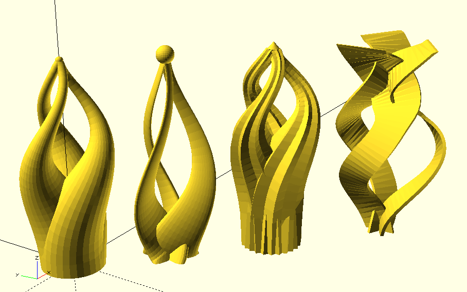
Here are the associated instantiations of the variants in figure 9.:
// Number 1
flames( 180 ) {
    circle( d = 60 , $fn = 30);
    sphere( d = 60 );
}

// Number 2
translate( [60, -60, 0] )
flames(
    180,
    steepness         = 0.1,
    transition        = 0.3,
    height_distortion = 1.2,
    slices            = 30
) {
    scale( [1, 0.33] )
    circle( d = 60 , $fn = 30);
    sphere( d = 120 );
}

// Number 3
union(){
    translate( [125, -125, 0] )
    flames(
        180,
        scaling_start     = [1.0, 1.0, 1.0],
        scaling_end       = [0.2, 0.2, 0.2],
        steepness         = 0.3,
        transition        = 0.35,
        height_distortion = 0.5,
        slices            = 30
    ) {
        square( 40, center = true);
        cylinder( d1 = 50, d2 = 0, h = 30);
    }

    translate( [125, -125, 0] )
    flames(
        180,
        scaling_start     = [1.0, 1.0, 1.0],
        scaling_end       = [0.2, 0.2, 0.2],
        steepness         = 0.3,
        transition        = 0.35,
        height_distortion = 0.5,
        slices            = 30
    ) {
        rotate( [0, 0, 45] )
        square( 40, center = true);
        cylinder( d1 = 50, d2 = 0, h = 30);
    }
}

// Number 4
translate( [200, -200, 0] )
flames(
    180,
    scaling_start     = [0.6, 0.6, 1.0],
    scaling_end       = [0.4, 1.0, 1.0],
    x_radius          = 25,
    y_radius          = 15,
    steepness         = 0.8,
    transition        = 0.6,
    height_distortion = 0.8,
    turns = 1.3,
    slices            = 50
) {
    square( [5, 45], center = true);
}